Optimal control of buoyancy-driven liquid steel stirring modeled with single-phase Navier–Stokes equations

Abstract

Gas stirring is an important process used in secondary metallurgy. It allows to homogenize the temperature and the chemical composition of the liquid steel and to remove inclusions which can be detrimental for the end-product quality. In this process, argon gas is injected from two nozzles at the bottom of the vessel and rises by buoyancy through the liquid steel thereby causing stirring, i.e., a mixing of the bath. The gas flow rates and the positions of the nozzles are two important control parameters in practice. A continuous optimization approach is pursued to find optimal values for these control variables. The effect of the gas appears as a volume force in the single-phase incompressible Navier–Stokes equations. Turbulence is modeled with the Smagorinsky Large Eddy Simulation (LES) model. An objective functional based on the vorticity is used to describe the mixing in the liquid bath. Optimized configurations are compared with a default one whose design is based on a setup from industrial practice.

1 Introduction

To produce steels with a high level of purity, companies employ a process called ladle gas stirring. It consists of mixing the liquid steel by injecting a noble gas from one or several nozzles located at the bottom of the vessel. The resulting buoyancy-driven stirring enhances the removal of inclusions (e.g., gaseous particles), the homogenization of the alloying materials in the steel, and the homogenization of the bath temperature [1]. A proper control of the stirring allows higher levels of cleanness of the steel grades, an increased production capacity through the reduction of the treatment time, and a decrease of the energy cost through the reduction of gas consumption.

In order to optimize the process parameters, experimental and numerical models of ladle stirring have been extensively used in the metallurgy literature. Usual parameters influencing the flow pattern are, e.g., the ladle geometry, the number and position of the nozzles, and the gas flow rates. The efficiency of the stirring is often described by the mixing time or the liquid circulation rate [1]. In [2], the authors use a two-phase model to study the effect of the height/diameter ratio on the mixing time and the liquid circulation rate. They showed that these two criteria are inversely proportional to each other and suggested that both quantities can be used equivalently as a criterion for the mixing efficiency. Furthermore, an aspect ratio of around 1.5 was found to lead to the most efficient mixing in axisymmetrical ladles, e.g., with one central nozzle. In [3], a simplified single-phase numerical model is applied to investigate the effect of different ladle geometries, nozzle positions, and gas flow rates on the mixing time. It was found that an off-center position of the nozzle and inclined ladle walls reduce the mixing time, thus improving the stirring efficiency. Another single-phase model is used in [4] to study the effect of two different nozzle configurations. An angle of 120^∘ between the two nozzles, instead of 150^∘, increases the circulation rate and decreases the volume of dead zones, i.e., areas of very small velocity. Multi-phase models with experimental measurements have been employed in [5] and [6]. The first paper investigated the optimum nozzle positions among a discrete number of configurations, while the second one studied the effect of the inflow location on the wear of the ladle wall in four cases.

More recent works focused on the profile of the injected gas flow rates rather than on the ladle geometry and the nozzles’ location. A pulsed stirring has been investigated numerically, experimentally, and industrially in [7]. Contrary to standard processes, they considered one bottom injection and one high-velocity lance injection from the side of the ladle. In practice, both use a constant gas flow rate. However, the authors showed that a pulsed lance stirring with a constant bottom gas injection can lead to a reduction of gas consumption while achieving the same steel quality with the same mixing time. This new injection profile has been successfully implemented in a plant. In [8], a bottom stirring with constant, but different, flow rates for each nozzle has been studied. Numerical and experimental results showed that the mixing time can then be significantly decreased.

In a major part of the literature, optimization studies consist in varying a small number of parameters (ladle geometry, gas nozzle position, gas flow rates, etc.) over a small, discrete set of values, and comparing the stirring performance, e.g., the mixing time. However, optimal control problems in the sense of continuous optimization have still to be explored in this area. Such problems require a computationally efficient state model, i.e., ladle stirring model, as well as relevant objective functionals.

As described in [9], optimization problems solve repeatedly the considered process with slightly changing coefficients. The needed time and memory usage for solving one state problem should be thus kept comparatively small in order to allow a reasonable computational cost for the whole optimization process. From this point of view, the use of multi-phase models for ladle stirring is not advisable. In addition to the Navier–Stokes equations, they require one additional convection equation for mixture models or a second set of Navier–Stokes equations for Euler–Euler models, [10]. On the contrary, the single-phase approach seems to be more appropriate because it is restricted to the incompressible Navier–Stokes equations [9]. The effect of gas stirring is modeled as a buoyancy force in the right-hand side of the momentum partial differential equation (PDE). Furthermore, [9] and [11] compared their numerical results with experimental measurements and showed that it can describe the bulk liquid flow satisfactorily in both quantitative and qualitative aspects.

On the other hand, the objective functional should describe the stirring efficiency, where also the cost for achieving the stirring are contained in this notion. The usual criterion for the stirring, i.e., the mixing time, introduces further difficulties such as a convection-dominated transport equation and the coupling with the flow equations. Alternatively, [12] and [13] use the vorticity to describe the mixing of the flow.

The objective of this paper is to study an optimal flow control problem in the context of buoyancy-driven ladle stirring, using a single-phase approach and the vorticity as a quantity to measure the efficiency of the mixing. In particular, it focuses on optimizing the gas flow rates as a function of time for fixed nozzle positions and of the two nozzle positions for fixed gas flow rates. Because of the unavailability of data for real steel ladles, the setup used in this paper is based on a laboratory-scale model of a real ladle, for which experimental studies were performed in [14, 15]. To perform the numerical simulations, an in-house research code for computational fluid dynamics (CFD) simulations [16, 17] is coupled with a freely available library for optimization [18]. The popular Smagorinsky large eddy simulation (LES) model is used for turbulence modeling. To numerically solve the optimization problems, a gradient-free routine is used. This approach avoids the solution of the adjoint problem, which is a convection-dominated problem backward in time, to compute the gradient, see [11, Sect. 4.3.3] for the derivation of this problem. To the best of our knowledge, the present paper is the first one that utilizes approaches from continuous optimization to find improved configurations for liquid steel stirring in a ladle.

The basic approach pursued in this paper has the advantage that it does not require very specialized software, such that it can be utilized by a wide community. In principle, any code that can simulate turbulent flows and any code for gradient-free optimization can be coupled. Just an interface has to be developed that transfers the necessary information between the codes. In fact, it is even not necessary to possess a deeper knowledge on the numerical methods implemented in these codes. However, one should be aware that the computational results will depend on the concrete turbulence model and probably on the used optimization routine. The first aspect will be already demonstrated in this paper by presenting results for different constants in the Smagorinsky LES model.

The modeling assumptions and the definition of the optimal control problem are presented in Sect. 2. Implementation aspects are described in Sect. 3 and the numerical studies and results in Sects. 4 and 5. Finally, a summary and an outlook are given.

2 The model for the optimization problem

2.1 The state model

The state model describes the flow in the ladle. The geometry corresponds to a laboratory-scale physical model of real ladles [14, 15]. Such experimental vessels employ water instead of steel and they are designed to describe the actual stirring using the Froude number as a similarity criterion, see [8, 19]. They provide velocity measurements which are important to validate the numerical results. The geometry as well as relevant entities in the definition of the buoyancy force are illustrated in Fig. 1 and the parameters of the model are listed in Table 1.

Figure 1

Relevant entities in the definition of the buoyancy force. Top left: Sketch of the 3d ladle with two eccentric nozzles; top right: The function $r_{c}$; bottom: The functions $\gamma _{i}(\cdot,z)$ (left) and $\alpha _{i}(\cdot,x,y,z)$ (right) for a constant gas flow rate $Q_{i}=17~{\mathrm{l}.\mathrm{min}^{-1}}$ (as in Table 1), where $r_{xy}$ is the horizontal distance to the nozzle, i.e., $r_{xy}^{2}=(x-x_{ni})^{2}+(y-y_{ni})^{2}$

Table 1 Default parameters of the 3d ladle stirring model from [9]. The value for Q is used as maximal value in the numerical studies presented here

Let Ω denote the domain of the ladle with boundary ∂Ω, outward pointing unit normal n and orthonormal tangential vectors $\boldsymbol{t}_{i}$, $i=1,2$ at ∂Ω, and let T be the final time. The upper part ${\Gamma _{\mathrm{top}}}$ of the boundary ∂Ω is the surface of the modeled fluid. Given an initial velocity field ${\boldsymbol{u}}^{0}({\boldsymbol{x}})$, the behavior of the flow is described by the incompressible single-phase Navier–Stokes equations where the effect of the rising gas is modeled by a buoyancy force on the right-hand side of the momentum equation, [9]:

$$\begin{aligned} &\partial _{t}{ \boldsymbol{u}}+( {\boldsymbol{u}}\cdot \nabla ) { \boldsymbol{u}}+ \nabla p - 2 \nabla \cdot \bigl( \operatorname{Re}^{-1}\mathbb{D}({ \boldsymbol{u}}) \bigr) = \bigl(1-( \alpha _{1}+\alpha _{2} ) \bigr) \boldsymbol{g} \quad{\text{in $(0,T] \times \Omega $}}, \\ &\nabla \cdot {\boldsymbol{u}} = 0 \quad{\text{in $(0,T] \times \Omega $}}, \\ &{\boldsymbol{u}}= {\boldsymbol{0}} \quad\text{in $(0,T] \times (\partial \Omega \setminus {\Gamma _{\mathrm{top}}}) $}, \\ &{\boldsymbol{u}}\cdot \boldsymbol{n} = 0 \quad{\text{in $(0,T] \times {\Gamma _{\mathrm{top}}}$}}, \\ &\boldsymbol{n}^{T} \mathbb{S} \boldsymbol{t}_{i} = 0,\quad i=1,2,{\text{ in $(0,T] \times {\Gamma _{\mathrm{top}}}$}}, \\ &{\boldsymbol{u}}(0,{\boldsymbol{x}}) = {\boldsymbol{u}}^{0}({ \boldsymbol{x}}) \quad{\text{in $\Omega $}}, \\ &\int _{\Omega } p \,{ \mathrm {d}{\boldsymbol {x}}}= 0 \quad{\text{in $[0,T]$}}, \end{aligned}$$

(1)

with

$$\begin{aligned} &\alpha _{i}(t,x,y,z) = \gamma _{i}(t,z) \exp \biggl( -2 \biggl( \frac{(x-x_{ni})^{2} + (y-y_{ni})^{2}}{r_{c}(z)^{2}} \biggr) ^{2} \biggr) , \\ &\gamma _{i}(t,z) = \frac{1}{2} \textstyle\begin{cases} \frac{U_{P_{i}}(t) }{U_{S}} +1 & \text{if } z\leq z_{C_{i}}, \\ \frac{U_{P_{i}}(t) }{U_{S}} + 1 -\sqrt{ ( \frac{U_{P_{i}}(t)}{U_{S}} +1 ) ^{2} - \frac{4Q_{i}(t)}{\pi r_{c}^{2}(z)U_{S}} } & \text{if } z\geq z_{C_{i}}, \end{cases}\displaystyle \\ &U_{P_{i}}(t) = \frac{4.4H^{1/4}}{R_{\mathrm{bot}}^{1/4}} Q_{i}^{1/3}(t),\quad i=1,2. \end{aligned}$$

Unknown quantities in (1) are the velocity u, $[{\mathrm{m}/\mathrm{s}}]$, and the pressure p, $[{\mathrm{Nm}/\mathrm{kg}}]$, which is actually the physical pressure divided by the density of the fluid. The coefficient on the right-hand side $\boldsymbol{g} = -(0,0,9.81)^{T}~{\mathrm{m}/\mathrm{s}^{2}}$ is the gravity. Further, the velocity deformation tensor $\mathbb{D}({\boldsymbol{u}}) = (\nabla {\boldsymbol{u}}+\nabla { \boldsymbol{u}}^{T})/2$ is the symmetric part of the velocity gradient and the stress tensor is given by $\mathbb{S} = \operatorname{Re}^{-1} \mathbb{D}({\boldsymbol{u}}) - p\mathbb{I}$, where $\mathbb{I}$ is the identity operator. For details of the modeling of the buoyancy force, it is referred to [9] and the references therein. The parameters of the coefficients that describe the buoyancy force are provided in Table 1. The quantities $Q_{i}(t)$ and $U_{P_{i}}(t)$, $i=1,2$, are the gas flow rates and the corresponding plume velocities at both nozzles, whose default values are given in Table 1. The critical heights

$$\begin{aligned} z_{C_{i}}(t) = \frac{1}{\tan (\chi )} \biggl(\sqrt{ \frac{4Q_{i}(t)}{\pi U_{S} (\frac{U_{P_{i}}(t)}{U_{S}} +1 )^{2}}} \biggr)-a,\quad i=1,2, \end{aligned}$$

are defined by the modeling procedure. For $z\ge z_{C_{i}}$, a closed-form formula can be derived from the so-called drift-flux model [20], which is then extended to small heights as given above. The positions of the nozzles are given by $x_{ni}$ and $y_{ni}$. Finally, the expansion of the gas plume radius with the height is given by $r_{c}(z) = \tan (\chi )(z+a)$.

It should be noted that the consideration of a fixed surface at $\Gamma _{\mathrm{top}}$ is a modeling assumption of single-phase models that simplifies the numerical setup. It has been observed in [9] that the fixed surface assumption works fine for ladles where the mixing is not too strong such that the top surface is relatively stable. The flow velocity obtained by this single-phase model was in good agreement with experimental measurements, although close to the surface there is more discrepancy. Since the zone of interest for the mixing is the whole domain, especially the bottom part with the dead zones, the single-phase model with fixed top surface is, in our opinion, an appropriate model for the studied optimal control problem.

For the numerical simulations, the Navier–Stokes equations (1) were converted to a non-dimensional form using the characteristic length scale $L=1~{\mathrm{m}}$ and the characteristic velocity scale $U=1~{\mathrm{m}/\mathrm{s}}$. The Reynolds number of the flow, based on these scales, the density of steel $\rho \approx 6980~{\mathrm{kg}/\mathrm{m}^{3}}$ and its dynamic viscosity $\mu \approx 2.7\cdot 10^{-3}~{\mathrm{Pa}\ \mathrm{s}}$, is given by

$$\begin{aligned} \mathrm{Re} = \frac{UL\rho }{\mu } \approx 2.6\cdot 10^{6}. \end{aligned}$$

(2)

This number, which is used in the dimensionless equations (1), indicates that the flow is turbulent. It is well known that its numerical simulation requires the usage of a turbulence model. We used the popular Smagorinsky large eddy simulation model [21], which adds to the momentum balance of the Navier–Stokes equations (1) the term

$$\begin{aligned} - 2 \nabla \cdot \bigl( \nu _{T} \mathbb{D}({ \boldsymbol{u}}) \bigr) \quad\text{with } \nu _{T} = C_{S} \delta ^{2} \bigl\| \mathbb{D}( { \boldsymbol{u}}) \bigr\| _{F}, \end{aligned}$$

(3)

where $\nu _{T}$ is called turbulent viscosity or eddy viscosity, δ is the filter width that is connected to the local mesh width, $\| \mathbb{D}( {\boldsymbol{u}}) \|_{F}$ is the Frobenius norm of $\mathbb{D}( {\boldsymbol{u}})$, and $C_{S}$ is the user-chosen Smagorinsky constant. In our simulations, the local filter width was set to be $2h_{K}$, where $h_{K}$ is the diameter of the mesh cell K. Typical values for the Smagorinsky constant are $C_{S} \in [0.0005,0.02]$, e.g., see [22]. Values from this range were utilized in our simulations.

2.2 The objective functional

The objective of the optimization study is to maximize the stirring efficiency, where the cost for performing the mixing is contained in this notion. As already discussed in the Introduction, there are several approaches for modeling the stirring efficiency. Here, a functional based on the vorticity $\mathbf {curl}({\boldsymbol{u}}) = \nabla \times {\boldsymbol{u}}$ of the flow will be used, inspired by [12, 13]. This functional, in combination with the singe-phase model for the flow, leads to optimization problems with reasonable complexity.

In the industrial practice, several aspects are often considered in terms of stirring efficiency. First, the stirring should be intense enough to remove the inclusions and homogenize the liquid bath. Furthermore, areas with a low circulation or no circulation at all, so-called dead zones, should be avoided. Finally, the gas consumption should be minimized during the process. Thus, we define the following objective functional to take into account these different aspects:

$$\begin{aligned} J({\boldsymbol{u}},Q_{1},Q_{2}) ={}& {-}\frac{\beta _{1}}{2} \int _{0}^{T} \bigl\lVert \mathbf {curl}({\boldsymbol{u}}) \bigr\rVert _{L^{2}(\Omega _{0})^{d}}^{2} \,{ \mathrm {d}t} \\ &{}+ \frac{\beta _{2}}{4} \int _{0}^{T} \bigl\lVert \max \bigl\{ \operatorname{curl}_{\mathrm{thr}} - \bigl\lVert \mathbf {curl}({\boldsymbol{u}})\bigr\rVert ^{2}, 0 \bigr\} \bigr\rVert _{L^{2}(\Omega )}^{2} \,{ \mathrm {d}t} \\ &{} +\frac{\lambda }{2} \int _{0}^{T} Q_{1}^{2}(t) + Q_{2}^{2}(t) \,{ \mathrm {d}t}, \end{aligned}$$

(4)

where $\beta _{1}\geq 0$, $\beta _{2} \geq 0$, $\lambda \geq 0$ are weights, $\operatorname{curl}_{\mathrm{thr}} > 0$ is a user-defined threshold parameter for the square of the Euclidean norm of the vorticity $\lVert \mathbf {curl}({\boldsymbol{u}})\rVert ^{2}$, and $\Omega _{0} \subseteq \Omega$.

The first integral represents a pure maximization of the curl of the velocity in $\Omega _{0}$. The cases $\Omega _{0} = \Omega$ and $\Omega _{0} \subsetneq \Omega$ are designated as the global and local maximization of vorticity, respectively. Since the first case measures an average quantity in the whole domain, it can allow locally for low vorticity. This is the reason why we introduced a subdomain $\Omega _{0}$: it can restrict the objective functional to areas which are known to be dead zones, for example near the bottom edge of the ladle. Thus, the second case ($\Omega _{0} \subsetneq \Omega$) is more likely to improve the vorticity in dead areas for appropriately chosen $\Omega _{0}$.

While the first integral is negative, the second term is positive. One finds by using Young’s inequality that $\lVert \mathbf {curl}({\boldsymbol{u}})\rVert _{L^{2}(\Omega _{0})^{d}}^{2} \le 2 \lVert \nabla {\boldsymbol{u}}\rVert _{L^{2}(\Omega _{0})^{d}}^{2}$. For the continuous problem, the energy dissipation $\mathrm{Re}^{-1} \int _{0}^{T} \lVert \nabla {\boldsymbol{u}}\rVert _{L^{2}( \Omega )^{d}}^{2}$ is bounded by the data of the problem due to the energy inequality. And also for the Smagorinsky model, it is known that $\mathrm{Re}^{-1} \int _{0}^{T} \lVert \nabla {\boldsymbol{u}}_{h}\rVert _{L^{2}( \Omega )^{d}}^{2}$ can be bounded by the data of the problem and the parameters of the model, e.g., see [22, Thm. 8.110]. Altogether, the first two terms are bounded for the continuous problem as well as for the discrete one. The integrand in the second term acts like a penalization: it has a positive contribution only where the vorticity is not high enough (namely, smaller than $\operatorname{curl}_{\mathrm{thr}}$), and the higher the gap between the vorticity and the required ‘threshold’ $\operatorname{curl}_{\mathrm{thr}}$, the higher the penalty. Physically, these areas correspond to dead zones. Where the vorticity is high enough (larger than or equal to $\operatorname{curl}_{\mathrm{thr}}$), it is 0. In other words, this functional takes into account the aspects ‘maximization of the vorticity’ and ‘reduction of dead zones’. Unlike the first integral, the whole domain Ω is considered in this term. Indeed, its integrand is zero where the vorticity is high. Thus, a local variant of the integral is not needed. One drawback is the Introduction of the additional variable $\operatorname{curl}_{\mathrm{thr}}$. It is not straightforward to fix physically relevant values for $\operatorname{curl}_{\mathrm{thr}}$, because there is no practical measurement or knowledge of how much the vorticity should be. In the numerical simulations presented below, several values for $\operatorname{curl}_{\mathrm{thr}}$ are tested and their impact on the optimal solution is studied.

Finally, the third integral describes the cost of the control, i.e., the gas consumption. Note that there is no cost related to the nozzles’ position $x_{n1}$, $y_{n1}$, $x_{n2}$, and $y_{n2}$. Indeed, the gas consumption is independent of the injection locations at the bottom of the vessel. When optimizing the nozzles’ position at constant gas flow rates, Sect. 5, the cost term is just a constant and consequently any value of λ leads to the same optimal configuration. We can thus assume $\lambda = 0$ in this case.

Altogether, the following cases are considered in the numerical studies:

• global maximization of vorticity $J_{1}$: $\beta _{1}=1$, $\beta _{2}=0$, and $\Omega _{0}=\Omega$,

• local maximization of vorticity $J_{2}$: $\beta _{1}=1$, $\beta _{2}=0$, and $\Omega _{0} \subsetneq \Omega$,

• regulation of vorticity $J_{3}(\operatorname{curl}_{\mathrm{thr}})$: $\beta _{1}=0$, $\beta _{2}=1$, and several values for $\operatorname{curl}_{\mathrm{thr}} \in [1,100]$.

2.3 Control variables

This paper presents two numerical studies which are of interest for the industrial practice. In the first one, the gas flow rates are optimized for fixed positions of the nozzles and the second one optimizes the nozzles’ positions for fixed gas flow rates. Thus, the physical control parameters are the two frequencies $\omega _{i}$ which are used for the parametrizations of the time-dependent gas flow rates $Q_{i}(t)$, and the nozzle positions $(x_{ni},y_{ni})$, for each nozzle $i \in \{1,2\}$.

Concerning the flow rates $Q_{1}(t)$ and $Q_{2}(t)$, lower and upper bounds are introduced to model limitations present in the application:

$$\begin{aligned} Q_{i}(t)& \in [ Q_{\mathrm{min}}, Q_{\mathrm{max}} ] = [1,17]~{ \mathrm{l}/\mathrm{min}} \quad\text{in $[0,T]$ for $i=1,2$}. \end{aligned}$$

(5)

In practice, the gas control system imposes restrictions on how often the valve can open and close within a second. In order to describe this situation realistically, we express $Q_{i}(t), i=1,2$, as

$$\begin{aligned} Q_{i}(t) = \frac{Q_{\mathrm{max}}+Q_{\mathrm{min}}}{2} + \frac{Q_{\mathrm{max}}-Q_{\mathrm{min}}}{2} \operatorname {sgn}\bigl( \sin ( 2\pi \omega _{i} t ) \bigr), \end{aligned}$$

(6)

which essentially switches between the minimum and maximum flow rate at a frequency $\omega _{i} \in [ \omega _{\mathrm{min}}, \omega _{ \mathrm{max}}]$. In our numerical studies, we used $\omega _{\mathrm{max}} = 0.5$ and the lower bound $\omega _{\mathrm{min}}$ is chosen such that $Q_{i}(t) = Q_{\mathrm{max}}$ for $t \in [0,T]$ is possible, which is the default case. In particular we set $\omega _{\mathrm{min}} = \omega _{\mathrm{max}}/T = 1/40$, since $T=20~{\mathrm{s}}$ is the final time in the optimization of the gas flow rates. The main reasons and goals why we chose to model the gas flow rates as in equation (6) are: (i) There is a small control space, concretely, there are only two variables with box-constraints, one for each nozzle. (ii) The gas flow should be maximal at the beginning, $Q(0)=Q_{\mathrm{max}}$, because the liquid steel is not at rest at $t=0$. (iii) This ansatz respects the practical boundaries, in particular the minimum and maximum flow rate and frequencies. (iv) It allows for $Q(t)=Q_{\mathrm{min}}$ at the end of the simulation, to save gas. (v) The flow rates should be either minimal or maximal, because intermediate values as well as smooth transitions are hard to realize in practice and would enlarge the control space. (vi) Equation (6) is a general description of pulsed flow rates, such as the one used in [7]. It can thus be used to verify whether a pulsed flow can generate a better stirring than a constant one.

The position of each nozzle i is determined, due to the cylindrical shape of the ladle, by a radius $r_{i}$ and an angle $\theta _{i}$:

$$\begin{aligned} &x_{ni} = r_{i} \cos ( \theta _{i} ),\qquad y_{ni} = r_{i} \sin ( \theta _{i} ), \\ &r_{i} \in [ 0, R_{\mathrm{bot}} ],\qquad \theta _{i} \in [0,2\pi ], \quad i=1,2. \end{aligned}$$

Note that $R_{\mathrm{bot}}$ is the bottom radius of the ladle, see Table 1. The rotational symmetry of the domain allows for some simplifications: Without loss of generality, we fix the angular position of one nozzle, $\theta _{1}=0.75\pi ={135}^{\circ}$ as in the default case, and restrict the second angle to be in one half of the circular bottom of the ladle, $\theta _{2}\in [\theta _{1}, \theta _{1}+\pi ]$. Therefore, the space of admissible controls for the nozzles has three dimensions instead of four. To further reduce the number of equivalent configurations, we also assume $r_{1} \ge r_{2}$. In order to avoid non-constant constraints¹ on the control space, we parameterize as follows:

$$\begin{aligned} \xi, \eta \in [0,1]\quad \text{and}\quad \theta _{2} \in [ 0.75\pi, 1.75 \pi ], \end{aligned}$$

with

$$\begin{aligned} r_{1} = R_{\mathrm{bot}} \textstyle\begin{cases} \xi + \eta /2 & \text{if } \xi + \eta \le 1, \\ \xi /2 + 1/2 & \text{else,} \end{cases}\displaystyle \qquad r_{2} = R_{\mathrm{bot}} \textstyle\begin{cases} \eta /2 & \text{if } \xi + \eta \le 1, \\ \xi /2 + \eta - 1/2 & \text{else.} \end{cases}\displaystyle \end{aligned}$$

In summary, the nozzles’ positions are described by the tuple $(\xi, \eta, \theta _{2})$ in the admissible set $[0,1]^{2} \times [0.75 \pi, 1.75 \pi ]$.

Remark 1

In [11, Sect. 4.5.3], results for modeling the controls $Q_{i}$, $i=1,2$, as functions of time that might change in every time step are presented. For those simulations, a flow field with $\mathrm{Re} = 96{,}000$ was used, which is much less turbulent than the flow field considered here. It was observed that most optimization processes stopped with the maximal number of iterations (500) and thus did not converge. The remaining simulations often proposed an oscillatory behavior of the controls, which cannot be realized in practice. And finally, the reductions of the cost functionals were often small compared with even a constant control. For these reasons, we were by far not satisfied with the numerical results from [11] and decided to reduce the complexity of the optimization problem such that it becomes considerably simpler, but not as simple as using a constant control for the gas flow rates.

3 Setup of the numerical studies

All flow simulations were performed with the in-house research code ParMooN, [16, 17], which is a finite element code. To perform the optimization, the freely available library NLopt [18] was coupled to ParMooN.

NLopt offers a number of gradient-free optimization routines. In preliminary studies, we tested several of them and decided to apply the constrained optimization by linear approximation (COBYLA) [23] for the simulations presented in this paper. Note that gradient-based optimization routines, which are likely to need less iterations than gradient-free routines, require the efficient evaluation of the gradient of the objective functional with respect to the control variables. In principle, this task can be done by solving an adjoint problem. However, the simulation of the adjoint of the considered problem is computationally highly challenging, in particular due to the time dependency of the process in combination with the nonlinearity of the model as well as the turbulent character of the flow field. The study of this approach requires a considerable extension of the available CFD solver and it will be a topic of future research.

As temporal discretization, the Crank–Nicolson scheme with equidistant time steps was used. In each discrete time instant, a nonlinear system of equations has to be solved. This system was linearized with a standard fixed point iteration, a so-called Picard iteration. Each step of the Picard iteration leads to a linear saddle point problem. The linear saddle point problems were discretized with the Taylor–Hood pair of finite element spaces $P_{2}/P_{1}$, i.e., the velocity was approximated with continuous and piecewise quadratic functions and the pressure with continuous and piecewise linear functions. This pair of finite element spaces belongs to the most popular inf-sup stable pairs [22]. Based on our experience from [24], the flexible generalized minimal residual (GMRES) method [25] was used as iterative solver for the linear saddle point problems and a least squares commutator (LSC) preconditioner [26, 27] was applied. The Picard iterations were stopped if the Euclidean norm of the residual vector was below 10⁻⁵.

The domain was triangulated by tetrahedral meshes of different refinement, see Table 2 for details and Fig. 2 for a graphical representation. The meshes were generated by providing the mesh at the bottom of the ladle and extending it by a sandwich technique into the third coordinate direction. All simulations were performed on HP compute servers HPE Synergy with Intel(R) Xeon(R) Gold 6154 CPU, 3.00 GHz.

Figure 2

Triangulations of the ladle, meshes for levels 2, 3, and 4

Table 2 Mesh parameters. The abbreviation “Dof” refers to the number of degrees of freedom

Numerical results will be presented for different resolutions of the temporal and spatial discretizations and for several Smagorinsky constants $C_{S}$ from (3) in order to study the impact of these numerical parameters on the result of the optimization problem.

4 Optimization of the gas flow rates

This section presents numerical results for the optimization of the gas flow rates using the default nozzles’ positions. From the practical point of view, optimized gas flow rates can be realized with an automated valve control system. The default configuration of the nozzle positions is given in Table 1.

As described in Sect. 2.3, the gas flow rate $Q_{i}(t) \in \{1,17\}~{\mathrm{l}/\mathrm{min}}$ for each nozzle, $i\in \{1, 2\}$, is determined by the frequency $\omega _{i} \in [\omega _{\mathrm{min}}, \omega _{\mathrm{max}}] = [1/40, 1/2]$, see (6) for the precise formula. Thus, $\omega _{1}$ and $\omega _{2}$ are the control variables for this optimization. A non-zero initial condition was applied, which describes a fully developed flow field. The objective was indeed to optimize $Q_{i}(t)$ during stirring, and not from the state where the liquid is at rest. This situation corresponds to real applications: the stirring is often strong at the beginning, before the operator adjusts the gas flow to optimize it. In terms of numerical simulations, this approach avoids computing repeatedly the first phase of the flow, leading to shorter time ranges for the simulations and substantial savings in computational cost. The choice of the time range T and the initial condition ${\boldsymbol{u}}^{0}$ was as follows:

• pre-computations with ${\boldsymbol{u}}^{0} = \boldsymbol{0}$ and $Q_{i}(t) = Q_{\mathrm{max}}$, $i\in \{1,2\}$, were performed until $T=100\ {\mathrm{s}}$, for each configuration, i.e., each combination of Δt and $C_{S}$,

• the time average $\bar {{\boldsymbol{u}}}$ of the velocity field in the last $20~{\mathrm{s}}$ ($80-100~{\mathrm{s}}$) was computed to smooth the flow fluctuations in time due to turbulence, see Fig. 3 for an example of an averaged velocity field,

  Figure 3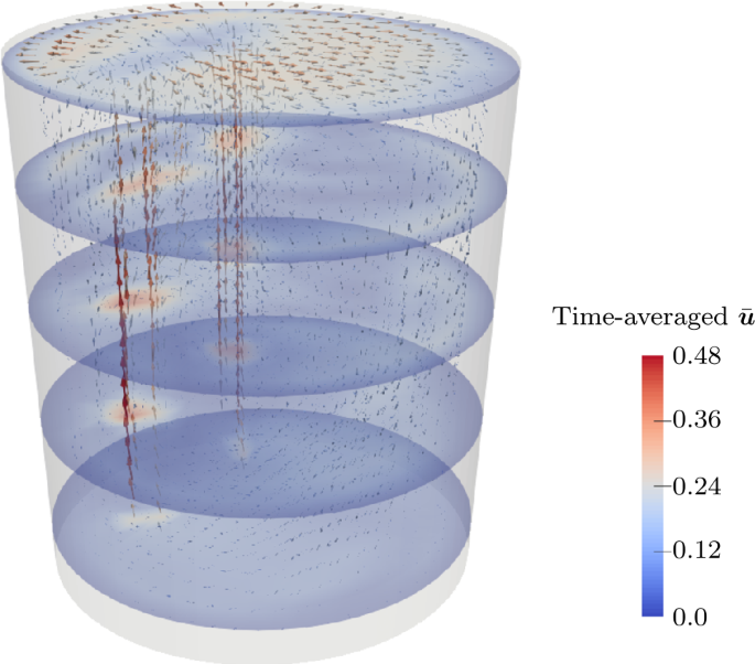

  

  Optimization of gas flow rates. Averaged velocity field $\bar {{\boldsymbol{u}}}$ obtained with $\Delta t=0.05$ and $C_{S}=0.005$. This solution is used as the initial condition ${\boldsymbol{u}}^{0}$ for the optimization studies which use the same Δt and $C_{S}$

• the optimization was performed with ${\boldsymbol{u}}^{0} =\bar {{\boldsymbol{u}}}$ and $T=20\ {\mathrm{s}}$, for each configuration.

Note that the optimal solutions obtained with this procedure might not be completely independent of ${\boldsymbol{u}}^{0}$, even if we considered a time-averaged initial flow field. The influence of the initial conditions on the optimal solution may be considered in future studies. Simulations within this study were performed on levels 2 and 3 of the spatial refinement, the time steps $\Delta t \in \{0.05, 0.025\}$, and the Smagorinsky constants $C_{S} \in \{0.005, 0.01, 0.02\}$.

Concerning the local maximization objective functional $J_{2}$, the subdomain $\Omega _{0}$ should contain regions where dead zones are expected, compare Sect. 2.2. Such regions are located in the lower part of the ladle away from the plume cones formed above of the nozzles. Therefore, $\Omega _{0}$ was defined to be the lower half of the domain excluding a box above the nozzles, as depicted in Fig. 4.

Figure 4

Optimization of gas flow rates. Subdomain $\Omega _{0}$ in the objective functional $J_{2}$ for the optimization of $Q_{i}$, $i\in \{1,2\}$. It covers the region where the dead zones are more likely to appear, i.e., the lower half of the domain $z \leq \frac{H}{2}$, excluding the area of the plume cones defined as a box ($-0.175 \leq x \leq -0.05$ and $-0.175 \leq y \leq 0.175$). This choice is suitable to avoid the high vorticity located close to the plume cones

Regarding the parameters in the objective functionals, the cost weight λ plays an important role for the optimization of the gas flow rates. Five values were studied: $\lambda = 10^{-i}$ for $i \in \{1, 2, 3, 4, 5\}$. For the sake of brevity, only results for two parameters $\operatorname{curl}_{\mathrm{thr}} \in \{1,100\}$ in the objective functional $J_{3}(\operatorname{curl}_{\mathrm{thr}})$ will be presented below.

To assess the effect of the optimization process for different combinations of spatial and temporal refinement and Smagorinsky constant, we defined a reduction $R \in [0,1]$ of the objective functionals for each simulation. Let $c_{\mathrm{min}}$ and $c_{\mathrm{max}}$ be the minimal and maximal values of the last part of the objective functional in equation (4), for which one finds with a straightforward but somewhat lengthy calculation

$$\begin{aligned} &c_{\mathrm{min}} = \min_{\omega \in [\omega _{\mathrm{min}},\omega _{ \mathrm{max}}]} \frac{1}{2} \int _{0}^{T} Q_{1}^{2}(t) + Q_{2}^{2}(t) \mathrm{d}t = 2900, \\ &c_{\mathrm{max}} = \max_{\omega \in [\omega _{\mathrm{min}},\omega _{ \mathrm{max}}]} \frac{1}{2} \int _{0}^{T} Q_{1}^{2}(t) + Q_{2}^{2}(t) \mathrm{d}t = 5780, \end{aligned}$$

with the flow rates $Q_{1}$ and $Q_{2}$ of the two nozzles, see equation (6). Then the reductions for the objective functionals $J_{1}$, $J_{2}$ and $J_{3}(\operatorname{curl}_{\mathrm{thr}})$ are defined by²

$$\begin{aligned} &R_{1} = \frac{J_{1}^{0} - \lambda c_{\mathrm{max}}}{J_{1}^{\mathrm{min}} - \lambda c_{\mathrm{max}}},\qquad R_{2} = \frac{J_{2}^{0} - \lambda c_{\mathrm{max}}}{J_{2}^{\mathrm{min}} - \lambda c_{\mathrm{max}}}, \\ &R_{3}(\operatorname{curl}_{\mathrm{thr}}) = \frac{J_{3}^{\mathrm{min}}(\operatorname{curl}_{\mathrm{thr}}) - \lambda c_{\mathrm{min}}}{J^{0}_{3}(\operatorname{curl}_{\mathrm{thr}}) - \lambda c_{\mathrm{min}}}, \end{aligned}$$

where $J_{1}^{0}, J_{2}^{0}, J^{0}_{3}(\operatorname{curl}_{\mathrm{thr}})$ are the initial values of the objective functionals and $J_{1}^{\mathrm{min}}, J_{2}^{\mathrm{min}}, J_{3}^{\mathrm{min}}(\operatorname{curl}_{ \mathrm{thr}})$ the respective results of the simulations.

Regarding the optimization solver, several stopping criteria were employed. Two criteria are related to the objective functional: its value ($\text{``stopval''}= -10^{10}$ for $J_{1}$ and $J_{2}$, 10⁻¹⁰ for $J_{3}(\operatorname{curl}_{\mathrm{thr}})$) and its reduction rate between the iterations (“ftol” =10⁻¹⁰). The difference of successive control variables was also used as a stopping criterion (“xtol” =10⁻⁵). Finally, the maximum number of iterations was fixed to be 200. All optimizations of gas flow rates terminated due to a sufficiently small difference of successive control variables.

A comparison of some results on mesh levels 2 and 3 for the same values of Δt and $C_{S}$ is presented in Table 3. It can be observed that usually the reductions of the objective functionals are rather similar. Since the simulations on the finer grid are likely to be more accurate, only results obtained on level 3 will be presented and discussed below.

Table 3 Optimization of gas flow rates. Reductions of the objective functionals, level 2 vs. level 3

Figure 5 provides some insight in the convergence history of the numerical optimization process. One can see that often a big reduction of the respective objective functional was achieved in the first one or two iterations. Usually, the optimization process converged after 25-40 iterations, compare also Tables 4 and 5, and took, on level 3 using the smaller time step $\Delta t=0.025$, on average 1.4 days, which corresponds to roughly 1.1 hours per iteration step. A general observation is that the higher the cost of injecting the noble gas, the higher is the reduction of the objective functional. Figure 5 gives also some information on the impact of the length of the time step. In most cases, the reductions of the objective functional were similar for both time steps. But there are some exceptions, in particular for $J_{2}$, where sometimes a considerably larger reduction is observed in case that the larger time step was used.

Figure 5

Optimization of gas flow rates. Reduction of the objective functionals during the optimization iteration, level 3, $C_{S} = 0.01$, different time steps

Table 4 Optimization of gas flow rates. Minimum objectives $M_{J, \lambda }$ and corresponding frequencies $\omega _{i}$, $i\in \{1,2\}$. The last column is the number of required optimization iterations. $\Delta t=0.05$, mesh 3

Table 5 Optimization of gas flow rates. Minimum objectives $M_{J, \lambda }$ and corresponding frequencies $\omega _{i}$, $i\in \{1,2\}$. The last column is the number of required optimization iterations. $\Delta t=0.025$, mesh 3

The main goal of the optimization consists in determining the gas flow rates $Q_{i}$, $i \in \{1,2\}$, for the nozzles. On mesh level 3 and with a given time step Δt, there are five values of the cost parameter λ, three values of the Smagorinsky constant $C_{S}$, and four objective functions, i.e., altogether 60 simulations. In contrast to the parameters for the temporal and spatial refinement, we have no guideline on how to define a Smagorinsky parameter that is in some sense the best choice. Thus, for each optimization parameter, i.e., $J \in \{J_{1}, J_{2}, J_{3}(1), J_{3}(100)\}$, and λ we considered the computed minimum objective value across all Smagorinsky constants $C_{S} \in \{0.005, 0.01, 0.02\}$:

$$\begin{aligned} M_{J,\lambda } = \min_{C_{S}} J\bigl({ \boldsymbol{u}}(J,\lambda,\Delta t,C_{S})\bigr), \end{aligned}$$

(7)

giving only 20 results.

Detailed results for both time steps are presented in Tables 4 and 5. First, one can observe that the predicted frequencies are sometimes different, most often $\omega _{1}$. In these cases, the frequency is often larger for the larger time step. As already mentioned, the reduction of the objective functionals was sometimes notably stronger for the larger time step. But most important, one can observe that the values of the objective functionals are usually smaller for the smaller time step, apart of the case of highly dominant costs $\lambda = 0.1$. Thus, the results for $\Delta t = 0.025$ are better and for this reason, we will restrict the further discussion to this time step.

Table 5 presents the obtained values $M_{J,\lambda }$ for $\Delta t = 0.025$. In this table, also the corresponding frequencies $\omega _{1}$ and $\omega _{2}$ of the gas flow rates are given, compare formula (5). The number of iterations for solving the optimization problem is for the simulation for which the given value $M_{J,\lambda }$ was obtained. A graphical representation of the optimal gas flow rates for the different combinations of objective functionals and parameters λ is provided in Fig. 6. It can be seen that in most cases the frequencies for the gas flow control of both nozzles are almost the same. Some notable exceptions are $J_{1}$ with $\lambda = 0.01$ and $J_{3}(1)$ with $\lambda = 0.0001$. In Fig. 6, it can be observed that for large cost parameters λ roughly half of the time the maximal gas flow rates are used and for the other half the minimal gas flow rates. For small parameters λ, often the whole time interval is operated with the maximal gas flow rates, sometimes with an exception of a short period at the end. It is remarkable that the switching between these two forms of controlling the gas flow rates occurs at smaller values of λ for the two functionals $J_{2}$ and $J_{3}(1)$ that were designed to pay particular attention to dead zones, i.e., to zones with low vorticity. One can also observe that the combination of a mostly constant and a pulsed flow rate can be found among the optimal solutions ($J_{1}$, $\lambda = 10^{-2}$). This approach was suggested in [7] for another type of stirring configuration, see Sect. 1.

Figure 6

Optimization of gas flow rates. Optimal gas flow rates for level 3, $\Delta t =0.025$, different objective functionals, and different parameters λ. The frequencies correspond to the values given in Table 5: blue: nozzle 1; red: nozzle 2

In our opinion, the obtained results meet the expectations from the qualitative point of view and they are in agreement with the default industrial practice ($Q_{i}(t) = Q_{\mathrm{max}}$, $i=1,2$, $t \in [0,T]$). In this respect, the studied objective functionals turned out to be reasonable choices.

5 Optimization of the nozzles’ positions

After having found that the used objective functionals and optimization approach lead to plausible results for the control of the gas flow rates, this section presents a numerical study where this strategy is applied to optimize the positions of the nozzles for fixed gas flow rates. This study can be regarded as a more conceptual study with respect to the industrial practice, since the change of the nozzles’ positions requires a re-design, and, consequently, a heavy investment, for new ladles. It is then particularly important that such a new design implies an improvement also for the conventional case of maximal constant inflow.

The optimization of the nozzles’ position considers the problem

$$\begin{aligned} \min_{\xi, \eta, \theta _{2}} J({\boldsymbol{u}},Q_{\mathrm{max}},Q_{ \mathrm{max}}), \end{aligned}$$

where the objective functional is defined in (4). As discussed in Sect. 2.2, the factor λ in the objective functional can be set to 0. Contrary to the previous study, the optimization of the nozzles’ position requires to start from a fluid at rest and to study the optimization over a period of time sufficiently long, until the flow is considered to be fully developed. Thus, at $t=0$, ${\boldsymbol{u}}^{0}={\boldsymbol{0}}$, and the end time is fixed to $T =60 {\mathrm{s}}$. Concerning the local maximization objective functional $J_{2}$, $\Omega _{0}$ cannot be chosen in such a special way as in the previous section, since the positions of the nozzles change. For the simulations presented below, $\Omega _{0}$ was set to be the lower half (with respect to its height) of the ladle. It corresponds to the region where dead zones are more likely to appear, for any position of the nozzles. The gas flow rate at both nozzles was the maximal rate $Q_{\mathrm{max}}$, given in Table 1.

Results obtained with the time steps $\Delta t \in \{0.05, 0.025\}$ in the Crank–Nicolson scheme will be presented. The constants used in the Smagorinsky LES model were $C_{S} \in \{0.005, 0.01, 0.02\}$. As initial positions of the nozzles, the default positions given in Table 1 were utilized, which corresponds to the parameters $r_{1}=r_{2}=0.1485~{\mathrm{m}}$, $\theta _{1}= 0.75\pi = {135}^{\circ}$, $\theta _{2} = 1.25\pi = {225}^{\circ}$. These positions are close to the positions of an industrially used ladle, which was investigated in [11]. The iteration for the optimization algorithm was controlled in the same way as for the optimization of the gas flow rates. Many simulations terminated again due to a sufficiently small difference in the successive control vectors. However, there were also two exceptions, which terminated only due to having reached the maximal number of iterations. In these cases, we could observe that the criterion of the difference of successive control vectors being small was almost satisfied. For this reason, we decided to include also these results below. Apart of these two cases, the optimization stopped usually after around 85 iterations. Altogether, the optimization of the position of the nozzles turned out to be considerably more difficult for the optimization routine than the optimization of the gas flow rates. On mesh 3 using the smaller time step size $\Delta t=0.025$, one computation took on average roughly 11 days (maximum about 24 days), which corresponds to approximately 3.1 hours per iteration step.

Our strategy was to perform the optimization procedures on levels 2 and 3 of the spatial refinement. These simulations were performed on a sequential computer. Then, after having identified good proposals for the control variables, these are compared on level 4 with pure flow simulations and evaluation of the objective functionals performed within a parallel framework.

As noted above, the objective functionals $J_{1}$ and $J_{2}$ are negative ($\lambda =0$) while $J_{3}(\operatorname{curl}_{\mathrm{thr}})$ is non-negative. In order to meaningfully compare their reductions with respect to the default configuration, we define the reductions $R_{i}$ as follows:

$$\begin{aligned} R_{1} = \frac{J_{1}^{0}}{J_{1}^{\mathrm{min}}},\qquad R_{2} = \frac{J_{2}^{0}}{J_{2}^{\mathrm{min}}},\qquad R_{3}(\operatorname{curl}_{ \mathrm{thr}}) = \frac{J_{3}^{\mathrm{min}}(\operatorname{curl}_{\mathrm{thr}})}{J^{0}_{3}(\operatorname{curl}_{\mathrm{thr}})}, \end{aligned}$$

(8)

where for each objective functional $J_{i}$, $i\in \{1,2,3\}$, its minimal computed value is $J_{i}^{\mathrm{min}}$ and its initial value (corresponding to the default configuration) is $J_{i}^{0}$. Therefore, the reductions are in the range of $[0,1]$, where 1 means no reduction. Then, given a number of simulation results $(x_{n1}^{k}, y_{n1}^{k})$ and $(x_{n2}^{k}, y_{n2}^{k})$ for the nozzle positions, we compute a weighted center as

$$\begin{aligned} (x_{ni,c}, y_{ni,c}) = \frac{\sum_{k} (x_{ni}^{k}, y_{ni}^{k}) (1-R^{k})}{\sum_{k} (1-R^{k})}. \end{aligned}$$

(9)

This quantity reduces the number of optimal solutions to investigate, similarly to $M_{J,\lambda }$, defined in equation (7).

Figure 7 presents the results for the functionals that maximize the vorticity, $J_{1}$ for the whole ladle and $J_{2}$ for the lower half of the ladle. On the top, results from level 2 are presented and on the bottom, results obtained on level 3. On the one hand, it can be observed that there are stronger reductions of the functionals on level 3. But on the other hand, it turns out that the predictions of the best positions for the nozzles (red cross and the given angle $\theta _{2}$) are qualitatively almost the same for $J_{1}$ and quite similar for $J_{2}$. We could observe a similar behavior also with respect to the other functionals: better reductions on level 3 and qualitatively quite close predictions of the optimal positions on both levels. For the sake of brevity, only the results computed on level 3 will be shown in the following pictures and discussed below.

Figure 7

Optimization of nozzles’ positions. Results obtained for levels 2 (top) and 3 (bottom), $J_{1}$ (left), and $J_{2}$ (right). The reduction of the functionals is depicted in accordance with the legend, i.e., the size of the circles represents $1-R_{i}$ with the corresponding reduction $R_{i}$ from equation (8). The red crosses are the computed weighted centers, see equation (9). The black plus signs indicate the default positions of the nozzles as given in Table 1

For the functional $J_{1}$, it is predicted that the nozzles should be nearly diametrically opposite to each other. The distance from the center of the ladle of the optimal positions is a little bit larger than the distance of the default positions. The optimal position of the second nozzle is somewhat different for $J_{2}$. First, it is closer to the center than in the default configuration. And second, it is not opposite to the first nozzle, however also not close to the default configuration.

The results for the regulation of the vorticity $J_{3}(\operatorname{curl}_{\mathrm{thr}})$, with different parameters $\operatorname{curl}_{\mathrm{thr}}$, are shown in Fig. 8. It can be seen that the higher $\operatorname{curl}_{\mathrm{thr}}$ the less the functionals are reduced. For all values of the parameter, the position of the first nozzle is proposed to be further away from the center of the ladle than in the default setting. For the other nozzle, $J_{3}(1)$, $J_{1}(25)$, and $J_{3}(50)$ predict a similar distance to the center, $J_{3}(10)$ a larger one, all compared with the default configuration. In all cases, a considerably larger angle between the nozzles is obtained than in the default setting.

Figure 8

Optimization of nozzles’ positions. Results obtained on level 3 for $J_{3}(\operatorname{curl}_{\mathrm{thr}})$ with $\operatorname{curl}_{\mathrm{thr}} \in \{1, 10, 25, 50\}$, top left to bottom right. The reduction of the functionals is depicted in accordance with the legend, i.e., the size of the circles represents $1-R_{i}$ with the corresponding reduction $R_{i}$ from equation (8). The red crosses are the computed weighted centers, see equation (9). The black plus signs indicate the default positions of the nozzles as given in Table 1

In summary, the optimization of all functionals proposes configurations that are clearly different to the default one and more or less close to diametrically opposite positions of the nozzle. The distances of the nozzles to the center of the ladle are similar to those in the default setting.

As already mentioned, simulations of the flow on refinement level 4 were performed for five of the optimal positions depicted in Figs. 7 and 8 with the red crosses. The data for these five positions are provided in Table 6. In addition, the default configuration, compare Table 1, was included in this study. The simulations were performed on 30 processors utilizing the Message Passing Interface (MPI) parallelization of the used CFD code. A small time step was chosen, $\Delta t=0.01$, and also a small Smagorinsky constant $C_{S}=0.0005$. We found that for larger constants, the Smagorinsky LES model was such diffusive that an almost steady-state solution was computed. For all five configurations, which were found to be optimal on mesh level 3 with respect to the different objective functionals, all objectives were evaluated for the simulations on level 4, thus allowing a comparison of the alternative configurations to the default one in terms of these objectives.

Table 6 Optimization of nozzles’ positions. Computed weighted centers (equation (9)) for the used objective functionals on level 3. The labels correspond to the configurations in Fig. 9

Figure 9 presents the results of this study, where the relative differences to the functional values obtained with the default configuration are used for assessment. It can be seen that for each alternative configuration there is a reduction of the corresponding objective functional on level 4, for which the configuration was optimized on level 3. All objective functionals, except $J_{1}$, are even reduced on all alternative configurations, i.e., all alternative configurations are better than the default one with respect to the objectives $J_{2}$, $J_{3}(1)$, $J_{3}(10)$, $J_{3}(25)$, and $J_{3}(50)$. The highest reductions, for all configurations, can be observed for $J_{2}$. For the industrial practice, it is also interesting to look at the solutions which give the highest reductions for all objective functionals. Computing the mean reductions, one finds that these are the solutions computed with the nozzles’ configurations proposed by $J_{2}^{\mathrm{opt},3}$ and $J_{3}^{\mathrm{opt},3}(1)$.

Figure 9

Optimization of nozzles’ positions. Relative differences of the objectives computed on mesh 4, i.e., the graph shows $(J_{\ast }-J_{\ast }^{\mathrm{default}})/ \lvert J_{\ast }^{\mathrm{default}} \rvert$. The numbers on top of the bars are the respective objective values for the default configuration

In summary, the optimization of the nozzles’ positions proposed for all objective functionals much different positions than the default one. The optimal positions are often rather close to an opposite arrangement of the nozzles. It was more difficult for the used optimization solver to converge than for the optimization of the gas flow rates. Flow simulations on a fine grid showed that in fact all objective functionals are reduced notably, compared with the default configuration, for the corresponding optimized positions found on the coarser grid.

6 Summary and outlook

This paper contains the first step of a continuous approach for optimizing buoyancy-driven liquid steel stirring. To the best of our knowledge, this is the first time that methods from continuous optimization have been used for this purpose. Two numerical studies were presented: the optimization of the gas flow rates for fixed nozzle positions (two control variables) and the optimization of the nozzles’ positions for fixed gas flow rates (three control variables). To perform the numerical simulations, two open source packages, a CFD code and an optimization library, were coupled. Turbulence modeling was necessary and a gradient-free optimization method was applied.

To describe the mixing of the flow field, an objective functional was defined that is based on the vorticity. Several special cases of this functional were considered. The optimal control of the gas flow rates turned out to depend on the cost for injecting the noble gas. Plausible results were obtained for all considered objectives. As a result of the optimizations of the nozzles’ positions, configurations were obtained that are close to an opposite arrangement of the nozzles, which is much different than the default configuration. Simulations on a fine grid showed that indeed all objective functionals gave better values for the corresponding alternative positions.

In fact, the current study can only be considered as a first step. For the near future, the investigation of alternative objective functionals and the use of more sophisticated turbulence models are realistic goals. A different control of the gas flow rates³ is possible as well as the combination of controlling the gas flow rates and the nozzles’ positions. Such studies increase the number of control variables and it remains to be seen how efficient a gradient-free optimization method behaves in these situations. Long term goals, which however increase the complexity of the numerical simulations enormously, are the use of a two-phase model for simulating the flow and the utilization of a gradient-based optimization method with the help of solving an appropriate adjoint problem.

References

Mazumdar D, Guthrie RIL. The physical and mathematical modelling of gas stirred ladle systems. ISIJ Int. 1995;35(1):1–20.
Turkoglu H, Farouk B. Mixing time and liquid circulation rate in steelmaking ladles with vertical gas injection. ISIJ Int. 1991;31(12):1371–80.
Zhu M-Y, Sawada I, Yamasaki N, Hsiao T-C. Numerical simulation of three-dimensional fluid flow and mixing process in gas-stirred ladles. ISIJ Int. 1996;36(5):503–11.
Goldschmit M, Owen AC. Numerical modelling of gas stirred ladles. Ironmak Steelmak. 2001;28(4):337–40.
Geng DQ, Lei H, He JC. Optimization of mixing time in a ladle with dual plugs. Int J Miner Metal Mater. 2010;17(6):709–14.
Llanos CA, Garcia S, Ramos-Banderas JA, Barreto JJ, Solorio G. Multiphase modeling of the fluidynamics of bottom argon bubbling during ladle operations. ISIJ Int. 2010;50(3):396–402.
Nadif M, Pusse C, Domgin JF, Bertoletti C, Perrin E, Sevilla D, Cantarini C. New stirring for an efficient steel desulfurization. In: The 6th European Oxygen Steelmaking Conference. Stockholm. 2011. p. 299–311.
Haiyan T, Xiaochen G, Guanghui W, Yong W. Effect of gas blown modes on mixing phenomena in a bottom stirring ladle with dual plugs. ISIJ Int. 2016;56(12):2161–70.
Najib A, John V, Ollila S. Revisiting the single-phase flow model for liquid steel ladle stirred by gas. Appl Math Model. 2019;67:549–56.
Ferziger JH, Perić M. Computational methods for fluid dynamics. 3rd rev. ed. Berlin: Springer; 2002.
Najib A. Optimal control of ladle stirring. Phd thesis, Department of Mathematics and Computer Science, FU Berlin, 2019.
Casas E. Optimality conditions for some control problems of turbulent flows. In: Flow control. IMA vol. math. Appl. vol. 68. Minneapolis, MN. 1992. New York: Springer; 1995. p. 127–47.
Bewley TR, Moin P, Temam R. DNS-based predictive control of turbulence: an optimal benchmark for feedback algorithms. J Fluid Mech. 2001;447:179–225.
Palovaara T, Visuri V-V, Fabritius T. Physical modelling of gas injection in a ladle. In: Proceedings of the 7th international congress on science and technology of steelmaking. 2018.
Alia N, Pylvänäinen M, Visuri V-V, John V, Ollila S. Vibrations of a laboratory-scale gas-stirred ladle with two eccentric nozzles and multiple sensors. J Iron Steel Res Int. 2019;26:1031–40.
Ganesan S, John V, Matthies G, Meesala R, Abdus S, Wilbrandt U. An object oriented parallel finite element scheme for computing pdes: design and implementation. In: IEEE 23rd international conference on high performance computing workshops (HiPCW) Hyderabad. New York: IEEE Press; 2016. p. 106–15.
Wilbrandt U, Bartsch C, Ahmed N, Alia N, Anker F, Blank L, Caiazzo A, Ganesan S, Giere S, Matthies G, Meesala R, Shamim A, Venkatesan J, John V. ParMooN—a modernized program package based on mapped finite elements. Comput Math Appl. 2017;74(1):74–88.
Johnson SG. The NLopt nonlinear-optimization package. 2019. http://ab-initio.mit.edu/nlopt.
Krishnapisharody K, Irons GA. A model for slag eyes in steel refining ladles covered with thick slag. Metall Mater Trans B. 2015;46(1):191–8.
Grevet JH, Szekely J, El-Kaddah N. An experimental and theoretical study of gas bubble driven circulation systems. Int J Heat Mass Transf. 1982;25(4):487–97.
Smagorinsky J. General circulation experiments with the primitive equations. Mon Weather Rev. 1963;91:99–164.
Volker J. Finite element methods for incompressible flow problems. Springer series in computational mathematics. vol. 51. Cham: Springer; 2016.
Powell MJ. A direct search optimization method that models the objective and constraint functions by linear interpolation. In: Advances in optimization and numerical analysis. Berlin: Springer; 1994. p. 51–67.
Ahmed N, Bartsch C, John V, Wilbrandt U. An assessment of some solvers for saddle point problems emerging from the incompressible Navier–Stokes equations. Comput Methods Appl Mech Eng. 2018;331:492–513.
Saad Y. A flexible inner-outer preconditioned GMRES algorithm. SIAM J Sci Comput. 1993;14(2):461–9.
Elman H, Howle VE, Shadid J, Shuttleworth R, Tuminaro R. Block preconditioners based on approximate commutators. SIAM J Sci Comput. 2006;27(5):1651–68.
Elman HC, Silvester DJ, Wathen AJ. Finite elements and fast iterative solvers: with applications in incompressible fluid dynamics. Numerical mathematics and scientific computation. 2nd ed. Oxford: Oxford University Press; 2014.
Acknowledgements
Not applicable.
Funding
Open Access funding enabled and organized by Projekt DEAL.
Author information
Authors and Affiliations
Contributions
The manuscript has been written, revised and edited by all authors. The involved programming has been done mainly by NA and UW. Conceptualization and literature studies were mostly done by NA and VJ. All authors read and approved the final manuscript.
Corresponding author
Ethics declarations
Ethics approval and consent to participate
Competing interests
The authors declare that they have no competing interests.
Consent for publication
Rights and permissions
Open Access This article is licensed under a Creative Commons Attribution 4.0 International License, which permits use, sharing, adaptation, distribution and reproduction in any medium or format, as long as you give appropriate credit to the original author(s) and the source, provide a link to the Creative Commons licence, and indicate if changes were made. The images or other third party material in this article are included in the article’s Creative Commons licence, unless indicated otherwise in a credit line to the material. If material is not included in the article’s Creative Commons licence and your intended use is not permitted by statutory regulation or exceeds the permitted use, you will need to obtain permission directly from the copyright holder. To view a copy of this licence, visit http://creativecommons.org/licenses/by/4.0/.
About this article
Cite this article
Wilbrandt, U., Alia, N. & John, V. Optimal control of buoyancy-driven liquid steel stirring modeled with single-phase Navier–Stokes equations. J.Math.Industry 11, 10 (2021). https://doi.org/10.1186/s13362-021-00106-7
Received:
Accepted:
Published:
DOI: https://doi.org/10.1186/s13362-021-00106-7