- Research
- Open access
- Published:
Multistep schemes for solving backward stochastic differential equations on GPU
Journal of Mathematics in Industry volume 12, Article number: 5 (2022)
Abstract
The Backward Stochastic Differential Equation (BSDE) is an important tool for pricing and hedging. Highly accurate pricing for low computation time becomes interesting for minimizing monetary loss. Therefore, we explore the opportunity of parallelizing high-order multistep schemes in option pricing. In the multistep scheme the computations at each space grid point are independent and this fact motivates us to select massively parallel GPU computing using CUDA. In our investigations we identify performance bottlenecks and apply appropriate optimization techniques to reduce the computation time in a uniform space domain. Runtime experiments manifest optimistic speedups for the parallel implementation on a single GPU, NVIDIA GeForce 1070 Ti.
1 Introduction
The backward stochastic differential equations (BSDEs) have been widely used in various areas such as physics and finance due to one of their key features, namely they provide a probabilistic representation of solutions of nonlinear parabolic partial differential equations (PDEs). We consider a (decoupled) forward backward stochastic differential equation (FBSDE) which has the form:
where \(X_{t}\), \(a \in\mathbb{R}^{n} \), b is a \(n\times d\) matrix, \(W_{t}\) is a d-dimensional Brownian motion, \(f (t,X_{t},y_{t},z_{t} ): [0,T ]\times \mathbb{R}^{n}\times\mathbb{R}^{m}\times\mathbb{R}^{m\times d} \to \mathbb{R}^{m}\) is the driver function and ξ is the terminal condition. For \(a = 0\) and \(b = 1\), namely \(X_{t} = W_{t}\), one obtains the standard BSDE of the form
where \(y_{t} \in\mathbb{R}^{m}\) and \(f (t,y_{t},z_{t} ): [0,T ]\times\mathbb{R}^{m} \times\mathbb{R}^{m\times d} \to\mathbb{R}^{m}\). The existence and uniqueness of the solution of (1) are proven in [20]. If \(dX_{t}\) in (1) is defined as the geometric brownian motion for modelling the asset price, and g is the payoff function of an European option, then (1) is related to the Black-Scholes PDE, see [14]. This is to say that \(y_{0}\) gives the option price and \(z_{t}/b\) represents the hegding portfolio, which presents the sensitivity of the option price \(y_{t}\) with respect to the asset price \(X_{t}\). This is called also Δ-hedging in the pricing theory.
Generally, it is rarely possible to find an analytical solution to a BSDE. Recently, many numerical methods have been thus proposed. For the numerical methods on spatial grids we refer to, e.g., [29–32]. The approaches based on the Fourier method for BSDEs are developed in [24, 25]. For probabilistic methods, Monte-Carlo approaches are investigated, e.g., in [10, 16], and tree-based methods in [6, 26]. And many others, see [1, 2, 4, 8, 9, 17].
Higher order numerical schemes demand usually more computing efforts, effective parallel implementations are thus in great demand. Some acceleration strategies based on Graphics Processing Unit (GPU) computing have been developed for the pricing problems in finance, however, a very little of them are BSDE-based approach. These works can be found in [7, 11, 22], where the acceleration strategies are applied on numerical methods of convergence order not higher than 2.
For higher order of convergence rate, the first multistep scheme on time-space grids is proposed in [32], where the resulting integrands by discretizing BSDE in time are approximated by using Lagrange interpolating polynomials. In [13], we have successfully parallelized that multistep scheme on GPUs, and showed the gain in computational time for option pricing via the Black-Scholes BSDE. However, the multistep scheme is only stable up to 3 multiple time levels due to Runge’s phenomenon. For a better stability and the admission of more time levels, a new multistep scheme is proposed in [27] by using spline instead of Lagrange interpolating polynomials. In principle, arbitrarily many multilevel time levels can be chosen in that multistep scheme, and in general the more time levels the higher accuracy. However, using more time levels also requires more computational cost. For this reason, in this work we investigate the massively parallel GPU computing in the multistep scheme [27], to make the scheme be more useful in practice. For example, a high accuracy for low computation time can minimize monetary loss in financial problems. An application that shows the importance of efficient approaches for pricing and the risk management of financial models can be found in [3].
The reminder of this paper is organized as following. In Sect. 2, we introduce the multistep method [27] for the numerical solution of BSDEs. Section 3 presents the algorithmic framework of the numerical method and the potential for preliminary reduction of computing time due to its special structure for uniform domains. In Sect. 4, we describe the GPU acceleration strategies for further reduction of computing time. Section 5 shows the numerical results including financial applications. Finally, we give the conclusions in Sect. 6.
2 The multistep scheme
In this section we introduce the multistep scheme [27] orientated to be parallelized on GPUs.
2.1 Preliminaries
Let \((\Omega,\mathcal{F},\mathbb{P},\{\mathcal{F}_{t}\}_{0\le t \le T} )\) be a complete, filtered probability space. In this space a standard d-dimensional Brownian motion \(W_{t}\) is defined, such that the filtration \(\{\mathcal{F}_{t}\}_{0\le t\le T}\) is the natural filtration of \(W_{t}\). We define \(|\cdot|\) as the standard Euclidean norm in the Euclidean space \(\mathbb{R}^{m}\) or \(\mathbb{R}^{m \times d}\) and \(L^{2} = L^{2}_{\mathcal{F}} (0,T; \mathbb{R}^{d} )\) the set of all \(\mathcal{F}_{t}\)-adapted and square integrable processes valued in \(\mathbb{R}^{d}\). Moreover, let \(\mathcal{F}_{s}^{t,x}\) for \(t\le s\le T\) be a σ-field generated by the Brownian motion \(\{x+W_{r}-W_{t},t\le r\le s\}\) starting from the time-space point \((t,x)\). We define \(E_{s}^{t,x} [X ]\) as the conditional expectation of the random variable X under the filtration \(\mathcal{F}_{s}^{t,x}\), i.e. \(E_{s}^{t,x} [X ]=E [X \vert\mathcal{F}_{s}^{t,x} ]\).
A pair of processes \((y_{t},z_{t} ): [0,T ]\times\Omega\to \mathbb{R}^{m} \times\mathbb{R}^{m \times d}\) is the solution of BSDE (1) if it is \(\mathcal{F}_{t}\)-adapted, square integrable, and satisfies (1) in the sense of
where \(f (t,X_{t}, y_{t},z_{t} ): [0,T ]\times \mathbb{R}^{m}\times\mathbb{R}^{n}\times\mathbb{R}^{m\times d} \to \mathbb{R}^{m}\) is \(\mathcal{F}_{t}\)-adapted and the third term on the right-hand side is an Itô-type integral. This solution exist under regularity conditions [20].
Let us consider the semilinear PDE
with the terminal condition \(u(T,x)=g(x)\). The following theorem can be obtained with a straightforward application of Itô’s lemma.
Theorem 1
(Nonlinear Feynman-Kac Theorem)
Let \(u \in C^{1,2}\) satisfying (4) and suppose that there exists a constant C such that \(|b(t,x)^{\top}D_{x} u(t,x)| \leq C(1+|x|)\) for each \((t,x) \in[0,T] \times\mathbb{R}^{m}\), then
is the unique solution of (1).
We note that the authors in [19] show the existence and uniqueness of a solution for BSDEs driven by a Lévy process with moments of all orders, which can be used for pricing in a Lévy market. The nonlinear Feynman-Kac formula for a general non-Markovian BSDE has been established in [21], where the path-dependent quasi-linear parabolic PDEs are considered. Furthermore, Feynman-Kac representation of fully nonlinear PDEs has been investigated, e.g., in [23].
2.2 The stable semidiscrete scheme
Let N be a positive integer and \(\Delta t = T/N\) the step size that partitions uniformly the time interval \([0,T ]\): \(0 = t_{0} < t_{1} < \cdots< t_{N-1} < t_{N} = T\), where \(t_{n} = t_{0} + n\Delta t\), \(n = 0,1,\dots,N\).
Let k and \(K_{y}\) be two positive integers such that \(1\le k \le K_{y} \le N\), which represent the number of time layers and interpolation points respectively. The BSDE (2) can be expressed as
Taking the conditional expectation \(E_{t_{n}}^{x}[\cdot]\) in (6) to obtain the adaptability of the solution and using cubic spline polynomial to approximate the integrand, the reference equation for y process reads (see the Appendix)
where \(R_{y}^{n}\) is the interpolation error. For the z process, using l and \(K_{z}\) instead of k and \(K_{y}\), multiplying both sides by \(\Delta W_{t_{n+l}}\) in (6) and taking the conditional expectation \(E_{t_{n}}^{x}[\cdot]\), the reference equation using cubic spline interpolation reads (see the Appendix)
where \(R_{z}^{n} = R_{z_{1}}^{n} + R_{z_{2}}^{n}\) are the interpolation errors. In [27], the authors have shown that the scheme is stable when
This is to say that the algorithm allows for arbitrary multiple time levels \(K_{y}\) and \(K_{z}\). Using the conditions of cubic spline interpolation to calculate the unknown coefficients, we have
with \(\gamma_{K_{y},j}^{K_{y}}\) and \(\gamma_{K_{z},j}^{1}\) representing the calculated coefficients of the cubic spline interpolation (Table 1 and Table 2 give the values up to 6 time levels). It is shown in [27] that the local errors in (7) are given by
provided that f and g are smooth enough. In (7) we need to divide by Δt to find the value of z process. Therefore, in order to balance time truncation errors, one might set \(K_{z} = K_{y}+1\).
The stable semidiscrete scheme for the d-dimensional case is given as follows: we denote \((y^{n},z^{n} )\) as the approximation to \((y_{t_{n}},z_{t_{n}} )\), given random variables \((y^{N-i},z^{N-i} )\), \(i = 0,1,\dots,K-1\) with \(K= \max\{K_{y},K_{z}\}\). Then \((y^{n},z^{n} )\) can be found for \(n = N-K,\dots,0\) such that
where \(y^{n} = (y^{n,\tilde{m}} )_{\tilde{m}\times1}\), \(z^{n} = (z^{n,\tilde{m},\tilde{d}} )_{\tilde{m}\times d}\), \(\Delta W_{t_{n+j}}^{\top}= (W_{t_{n+j}}^{\tilde{d}} )_{ \tilde{d}\times1} - (W_{t_{n}}^{\tilde{d}} )_{\tilde{d} \times1}\), \(\tilde{m}=1,2,\ldots,m\) and \(\tilde{d}=1,2,\ldots,d\). In the following, we only present the results of the error analysis, for their proofs we refer to [27] and [32].
Lemma 1
The local estimates of the local truncation errors in (7) satisfy
where \(C > 0\) is a constant depending on T, f, g and the derivatives of f and g.
Theorem 2
Suppose that the initial values satisfy
where \(K_{y} = 1, 2, 3\) for the first equation and \(K_{y} >3 \) for the second one. For a sufficiently small time step Δt it can be shown that
where \(C > 0\) is a constant depending on T, f, g and the derivatives of f and g.
Theorem 3
Suppose that the initial values satisfy
where \(K_{z} = 1, 2, 3\) for the first equation and \(K_{z} >3 \) for the second one, and the condition on the initial values in Theorem 2is fulfilled. For a sufficiently small time step Δt it can be shown that
where \(C > 0\) is a constant depending on T, f, g and the derivatives of f and g.
Remark 1
If f does not depend on process z, the maximum order of convergence for the y process is 4 and 3 for the z process; If f depends on process z, the maximum order of convergence for the y and z processes is 3.
2.3 The fully discrete scheme
Let Δx denote the step size in the partition of the uniform d-dimensional real axis, i.e.
where
Let \(x_{\mathbf{i}} = (x^{1}_{i_{1}}, x^{2}_{i_{2}}, \ldots, x^{d}_{i_{d}} )\) for \(\mathbf{i} = (i_{1}, i_{2}, \ldots, i_{d} ) \in \mathbb{Z}^{d}\). We denote \((y^{n}_{\mathbf{i}},z^{n}_{\mathbf{i}} )\) as the approximation to \((y_{t_{n},x_{\mathbf{i}}},z_{t_{n},x_{\mathbf{i}}} )\), given the random variables \((y^{N-l}_{\mathbf{i}},z^{N-l}_{\mathbf{i}})\), \(l = 0,1,\dots,K-1\) with \(K = \max\{K_{y},K_{z}\}\). Then \((y^{n}_{\mathbf{i}},z^{n}_{\mathbf{i}})\) can be found for \(n = N-K,\dots,0\) such that
where \(\hat{E}_{t_{n}}^{x_{i}} [ \cdot ]\) is used to denote the approximation of the conditional expectation. The calculations at each space grid point \(x_{\mathbf{i}}\) in (9) are independent, for each time layer \(t_{n}\). Therefore, the parallelization strategy is fully related with the space discretization, which will be discussed in the following Sections.
The functions in the conditional expectations involve the d-dimensional probability density function of the Brownian Motions, one can choose e.g., the Gauss-Hermite quadrature rule to achieve a high accuracy only with a few space points. The conditional expectation can be can be sufficiently accurately approximated by a clever table interpolation
where \(\hat{y}^{n+k}\) are interpolating values at the space points \((x_{\mathbf{i}}+\sqrt{2k\Delta t} a_{\Lambda} )\) based on \(y^{n+k}\) values, \((\omega_{\Lambda}, a_{\Lambda})\) for \(\Lambda= (\lambda_{1}, \lambda_{2},\ldots, \lambda_{d} )\) are the weights and roots of the Hermite polynomial of degree L (see [12]), \(\omega_{\Lambda}= \prod_{\tilde{d}=1}^{d} \omega_{\lambda_{ \tilde{d}}} \), \(a_{\Lambda}= ( a_{\lambda_{1}}, a_{\lambda_{2}},\ldots, a_{ \lambda_{d}} )\) and \(\sum_{\Lambda=1}^{L} = \sum_{\lambda_{1}=1,\ldots, \lambda_{d}=1}^{L, \ldots, L}\). In a similar way, one can express the other conditional expectations in (9).
3 The algorithmic framework
According to the numerical algorithm represented in Sect. 2, the whole process for numerically solving BSDEs can be divided into three steps.
-
1.
Construct the time-space discrete domain.
We divide the time period \([0,T]\) into N time steps using \(\Delta t = T/N\), i.e., \(N+1\) time layers, and the space domain \(\mathbb{R}^{d}\) using step size Δx (see also Sect. 2.3). We use the truncated domains \([-16, 16 ]\) and \([-8, 8 ]\) for the grid space, where the former is used for 1-dimensional examples and the latter for the 2-dimensional ones. Note that larger domain can be also used, however, the approximation will be not improved. This is to say that those truncated domains are sufficient for our numerical experiments. Furthermore, in order to balance the errors in time and space directions, we adjust Δx and Δt such that they satisfy the equality \((\Delta x)^{r}=(\Delta t)^{q+1}\), where \(q = \min \{ K_{y}+1,K_{z} \} \) and r denotes the global error from the interpolation method used to generate the non-grid points when calculating the conditional expectations. For a better illustration, we show a visualisation of the domain for \(K_{y} = K_{z} = 1\), \(d = 1\) in Fig. 1, including the non-grid points.
Figure 1 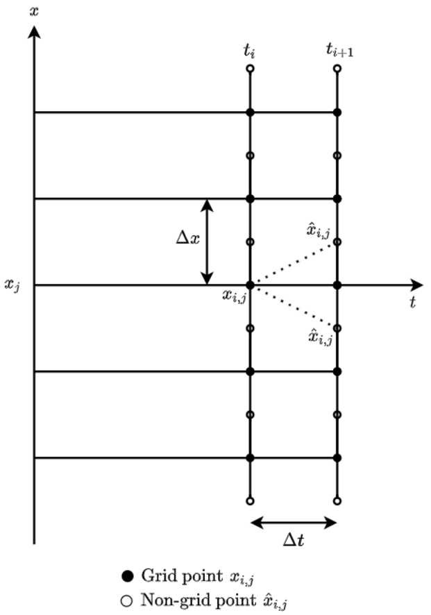
Time-space domain
-
2.
Calculate K initial solutions with \(\boldsymbol{K = \max\{K_{y},K_{z}\}}\).
Generally, only the terminal values are given and one needs to compute the other \(K-1\) initial values. To obtain these initial values, we start with \(K = 1\) and choose an extremely small time step size Δt.
-
3.
Calculate the numerical solution \(\boldsymbol{(y_{0}^{0},z_{0}^{0})}\) backward using equation (9).
Note that the calculation for the y process is done implicitly with Picard iteration.

In step 1, some of the generated non-grid points could be outside of the truncated domain (see Fig. 1). For these points, we take the values on the boundaries as approximations (constant extrapolation). Note that one could also do extrapolation for those points outside, however, a longer computation time will be needed. As mentioned in (10), we use interpolation to approximate the values for y and z at non-grid points. The computation time drawback when interpolating is finding the position of the new points in the interpolating process. A natural search algorithm is to loop over all the grid points, and find in which interval the point belongs to. In the worst case, an \(\mathcal{O} (M^{d} )\) work is needed. Fortunately, the structure of the Gauss-Hermite quadrature creates the symmetry for the non-grid points. Recall that each new point is generated as \(X_{\lambda_{\tilde{d}}} = x_{i_{\tilde{d}}} + \sqrt{2k\Delta t} a_{ \lambda_{\tilde{d}}}\). This means that taking \(\operatorname{int} (\frac{X_{\lambda_{\tilde{d}}}-x_{\min }}{\Delta x} )\) for \(x_{i_{\tilde{d}}} \in [x_{\min}, x_{\max} ]\) and \(M-\operatorname{int} (\frac{X_{\lambda_{\tilde{d}}}-x_{\min }}{\Delta x} )\) for \(x_{i_{\tilde{d}}} \in [x_{\max}, x_{\min} ]\) gives the left boundary of the grid interval that \(X_{\lambda_{\tilde{d}}}\) belongs to, with \(\operatorname{int}(x)\) giving the integer part of x. As a result, this step in the algorithm can be done in \(\mathcal{O} (d )\), i.e., without a for-loop. This benefit comes from the uniformity of the space domain. This substantially reduces the total computation time, as it will be demonstrated in the numerical experiments.
In step 2, we do not consider 2K (K for y and K for z) interpolations for each new calculation, but only 2. Suppose that we are at time layer \(t_{n-K}\). To calculate y and z values on this time layer, one needs the calculation of conditional expectations for K time layers. In our numerical experiments, we consider 1 and 2 dimensional examples, the higher dimensional problem can be parallelized for a device (GPU) with large memory. The cubic spline interpolation is used to find the non-grid values for 1-dimensional cases and bicubic interpolation for 2-dimensional cases. For instance, the coefficients for the y process are \(A_{y}\in\mathbb{R}^{K\times (4^{d} \times M^{d} )}\), all the coefficients are stored. When we are at time layer \(t_{n-K-1}\), only the spline interpolation corresponding to the previous calculated values is considered. Then, the columns of matrix \(A_{y}\) are shifted +1 to the right in order to delete the last column and enter the current calculated coefficients in the first column. The new \(A_{y}\) is used for the current step. The same procedure is followed until \(t_{0}\). This reduces as well the amount of work for the algorithm.
In the final step (step 3), we consider to merge calculation of conditional expectations in (9), which is important for the reduction of computation time in the parallel implementation. This will be mentioned in more details in the next Section.
4 Parallel algorithm
In this Section we present the parallelization strategy of the multistep scheme presented in the previous sections. Basically, we parallelize the problem straightforwardly, while keeping attention on the optimal Compute Unified Device Architecture (CUDA) execution model, i.e., creating arrays such that the access will be aligned and coalesced, reducing the redundant access to global memory, using registers when needed etc..
The first and second steps of the algorithm are implemented in the host. The third step, together with the operator for performing \(\mathcal{O} (d )\) work in the searching procedure of the interpolation and the idea of shifting coefficients of this procedure, are fully implemented in the GPU device. Recall from (9) that the following steps are needed to calculate the approximated values on each unknown time layer backward:
-
Generation of the non-grid points \(\boldsymbol{X_{\Lambda}= x_{\mathbf{i}} + \sqrt{2k\Delta t} a_{\Lambda}}\).
In the uniform space domain, the non-grid points need to be generated only once. To do this, a kernel is created where each thread generates \(L^{d}\) points (Gauss-Hermite points) for each space direction. This kernel adds insignificant computing time in the total algorithmic time.
-
Calculation of the values \(\hat{\boldsymbol{y}}\) and \(\hat{\boldsymbol{z}}\) at the non-grid points.
This is the most time consuming part of the algorithm, which is related with finding the corresponding interpolating functions for the given y and z points, in order to interpolate their values in the non-grid ones. For the 1-dimensional cases, we have considered the cubic spline interpolation. Since (9) involves the solution of two linear systems, the Biconjugate Gradient Stabilized (BiCGSTAB) [28] iterative method is used since the matrix is tridiagonal. For this, we consider the CUDA Basic Linear Algebra Subroutine (cuBLAS) and CUDA Sparse (cuSPARSE) libraries [5]. For the inner product, second norm and addition of vectors, we use the cuBLAS library. For the matrix vector multiplication, we use the cuSPARSE library with the compressed sparse row format, due to the structure of the system matrix. Moreover, we created a kernel to calculate the spline coefficients based on the solved systems. Finally, a kernel to apply the operator for the searching procedure of interpolation is created to find the values at non-grid points. Note that each thread is assigned to find \(m+m\times d\) values (m for y and \(m\times d\) for z). For the 2-dimensional examples, we have considered the bicubic interpolation. We need to calculate 16 coefficients for each point. Based on the bicubic interpolation idea, we need the first and mixed derivatives. These are approximated using finite difference schemes of the fourth order of accuracy (central for the interior points, forward and backward for the boundary points). Therefore, a kernel is created where each thread calculates these values. Moreover, to find the 16 coefficients, a matrix vector multiplication needs to be applied for each point. Therefore, each thread performs a matrix-vector multiplication using another kernel. Finally, a kernel to apply the operator for the searching procedure of interpolation is created to find the values at non-grid points, where each thread calculates \(m+m\times d\) values.
-
Calculation of the conditional expectations.
As mentioned above, we merge the calculation of conditional expectations. For the first conditional expectations in the right hand side of (9), we create one kernel, where each thread calculates one value by using (10). For the other ones, we merged their calculation (three conditional expectations) in one kernel, namely \(\hat{E}_{t_{n}}^{x_{\mathbf{i}}} [\hat{z}^{n+j} ]\), \(\hat{E}_{t_{n}}^{x_{\mathbf{i}}} [f(t_{n+j},\hat{y}^{n+j},\hat {z}^{n+j}) ]\) and \(\hat{E}_{t_{n}}^{x_{\mathbf{i}}} [f(t_{n+j},\hat{y}^{n+j},\hat {z}^{n+j}) \Delta W_{t_{n+j}} ]\), for \(j=1,2,\dots,K\). This reduces the accessing of data multiple times from the global memory and gives more work to the thread, such that it does not stay idle. Note that one thread calculates \(2\times m\times d + m\) values.
-
Calculation of the z values.
The second equation in (9) is used and each thread calculates \(m\times d\) values.
-
Calculation of the y values.
The first equation in (9) is used and each thread calculates m values, using the Picard iterative process.
In the next Section, we present some numerical examples to show the accelerated computation on GPU computing with applications in option pricing.
5 Numerical results
We implement the parallel algorithm using CUDA C programming. The parallel computing times (only for one run) are compared with the serial ones on a CPU. Furthermore, the speedups are calculated. The Central Processing Unit (CPU) is Intel(R) Core(TM) i5-4670 3.40Ghz with 4 cores, where only one core is used for the serial calculations. The GPU is a NVIDIA GeForce 1070 Ti with a total 8GB GDDR5 memory.
We choose the degree of the Hermite polynomial \(L = 32\) for the 1-dimensional examples and \(L = 8\) for the 2-dimensional ones. For the Picard interations, we choose \(p = 30\). With these values, the quadrature error and iteration error are so small that they won’t affect the convergence rate.
Example 1
Consider the nonlinear BSDE [32].
The analytic solution is
The exact solution with \(T=1\) is \((y_{0},z_{0} )= (\frac{1}{2},\frac{1}{4} )\). In Table 3, we show the importance of the proposed technique when interpolating non-grid values, for a high N. Note that the computation time is given in seconds. We see that without the operator to find the position of the non-grid points in space, the computation serial time is very high.
In Table 4, we present the results using 256 threads per block with \(K = K_{y} = K_{z}\), \(t_{0}=0\) and \(T = 1\). As mentioned before, the better accuracy can be archived by using a higher-step scheme. For \(K >3\), the errors decrease moderately due to Theorem 2. The higher the value of time layers N the more work can be assigned to the GPU, and the speedup of the application can thus be increased. The speed up also increases on a smaller magnitude for \(K>3\), since the number of space data points given from M is the same. These are visualized in the plots of \(\log_{10}(|y_{0,0}-y_{0}^{0}|)\), \(\log_{10}(|z_{0,0}-z_{0}^{0}|)\) and speedup with respect to N for \(K = 1, \ldots, 6\) in Fig. 2. The highest speedup (26×) is for the multistep scheme with \(K=6\) and \(N=1024\).

Plots of the results for Example 1
Example 2
Consider the nonlinear BSDE [32]
The analytic solution is
The exact solution with \(T=1\) is \((y_{0},z_{0} )= (\ln (3 ),\frac{1}{3} )\). The results using 256 threads per block with \(K = K_{y} = K_{z}\), \(t_{0}=0\) and \(T = 1\) are presented in Table 5. We conclude the same as in the previous example, except the fact that the accuracy is decreased. This is due to the convergence order given in Theorem 3, which reduces to be at most 3, since the driver function depends on the z process. Furthermore, we get higher speedup compared with previous example due to the more complicated driver function (i.e. more data are accessed, more special functional unit is used etc.). The speedup is 35×. We display the plots of \(\log_{10}(|y_{0,0}-y_{0}^{0}|)\), \(\log_{10}(|z_{0,0}-z_{0}^{0}|)\) and speedup with respect to N for \(K = 1, \ldots, 6\) in Fig. 3.

Plots of the results for Example 2
To optimize the application, we have used the following iterative approach:
-
1.
Apply a profiler to the application to gather information
-
2.
Identify application hotspots
-
3.
Determine performance inhibitors
-
4.
Optimize the code
-
5.
Repeat the previous steps until desired performance is achieved
We considered the case with \(N=1024\) and \(K_{y}=K_{z}=6\). To make the optimization process be more clear, we show the detailed information after each optimization iteration as follows.
-
In the first iteration of the optimization process, we gathered the application information using nvprof (NVIDIA Command-line Profiler). The results are presented in Table 6(a). The application hotspot is the \(nrm2\_\mathit{kernel}\) kernel, which calculates the second norm in the BiCGSTAB algorithm. This is already optimized. Therefore, to overcome this bottleneck, we used the dot kernel \(\mathit{dot}\_ \mathit{kernel}\). The computation time is reduced from 8.04 s to 0.86 s. The new speedup after the first iteration becomes 57× in stead of 35×.
Table 6 Results of iterative optimization process for Example 2 -
In the second iteration, the next bottleneck for the application is the kernel that calculates the non-grid values for process y and z (\(\mathit{sp}\_\mathit{inter}\_\mathrm{non}\_\mathit {grid}\_d\_\mathit{no}\_\mathit{for}\)) after each time layer backward. The performance of the kernel is limited by the latency of arithmetic and memory operations. Therefore, we considered loop interchanging and loop unrolling techniques. This reduced the computation time of the corresponding kernel and other kernels related with it, as shown in Table 6(b). By this, we reduced the computation time for \(\mathit{sp}\_\mathit{inter}\_\mathit{non}\_\mathit{grid}\_d\_ \mathit{no}\_\mathit{for}\) from 2.48 s to 1.16 s. By default, we have reduced the computation time from 2.28 s to 1.46 s for \(\mathit{calc}\_f\_\mathit{and}\_c\_\mathit {exp}\) (the kernel in the third item of Sect. 4) because we needed to change the way how the non-grid points are stored and accessed and also reduction for \(\mathit{calc}\_c\_\mathit{exp}\_d\) (calculates the conditional expectation) from 0.22 s to 0.04 s. The new speedup is 69×. It can be observed from Table 6(c) that again the application bottleneck is the same kernel. Therefore, it is not worth optimizing the application furthermore.
-
Finally, we decreased the block dimension from 256 threads to 128 in order to increase parallelism. The final speedup is 70×.
Example 3
Consider the Black-Scholes FBSDE [14]
For constant parameters (i.e. \(r_{t} = r\), \(\mu_{t} = \mu\), \(\sigma_{t}=\sigma\), \(\delta_{t} = \delta\)), the analytic solution for a call option is
where \(N (\cdot )\) is the cumulative standard normal distribution function. In this example, we consider \(T=0.33\), \(K=S_{0}=100\), \(r=0.03\), \(\mu=0.05\), \(\delta=0.04\) and \(\sigma=0.2\) (taken from [32]) with the solution \((y_{0},z_{0} ) \doteq (4.3671,10.0950 )\). Note that the terminal condition has a non-smooth problem for the z process. Therefore, for discrete points near the strike price K (also called at the money region), the initial value for the z process will cause large errors on the next time layers. To overcome this non-smoothness problem, we considered smoothing the initial conditions, cf. the approach of Kreiss [15]. For the forward part of Example 3, we used the analytic solution
In order to ensure a uniform stock price domain, we switch to the log stock price domain \(X_{t} = \ln (S_{t} )\). In Table 7 we show the importance of using this transformation.
The results using 256 threads per block with \(K = K_{y} = K_{z}\), \(t_{0}=0\) and \(T = 0.33\) are presented in Table 8. As in the previous BSDE examples, the highest accuracy is achieved for the maximal considered number of steps K and the number of time layers N, namely a 6-step scheme with \(N = 256\), where we also have the highest speedup of 12×. We draw the plots of \(\log_{10}(|y_{0,0}-y_{0}^{0}|)\), \(\log_{10}(|z_{0,0}-z_{0}^{0}|)\) and speedup with respect to N for \(K = 1, \ldots, 6\) in Fig. 4.

Plots of results for Example 3
Compared to the parallelized multistep scheme [32] in [13], the numerical results are more accurate, since we can considered \(K > 3\). Moreover, we optimized the kernels created for the Black-Scholes BSDE for \(N=256\) and a high K, namely \(K = K_{y}=K_{z}=6\). The optimization iteration process is the same as in Example 2. The final speedup is 31×. Note that this speedup is for 256 time layers. In Example 2, we optimized for 1024 time layers. The high accuracy \(\mathcal{O} (10^{-12} )\) with a high value of K can be achieved for more modest computation time then 6.47 seconds.
Obviously, it is more interesting to achieve the parallelization of higher dimensional BSDEs on the GPUs.
Example 4
We start with the 2-dimensional BSDE [30]
where \(W_{t} = (W_{t}^{1},W_{t}^{2} )^{\top}\), \(z_{t} = (z_{t}^{1},z_{t}^{2} )\), \(A = (\frac{1}{2},\frac{1}{2} )^{\top}\) and \(M = (1, 1 )\).
The analytic solution is
The exact solution with \(T=1\) is \((y_{0}, (z_{0}^{1},z_{0}^{2} ) )= (0, (1,1 ) )\). The results using 256 threads per block with \(K = K_{y} = K_{z}\), \(t_{0}=0\) and \(T = 1\) are presented in Table 9. Note that \(|z_{0,0}-z_{0}^{0}|\) in 2-dimensional case is given by \(\frac{1}{2} ( |z_{0,0}^{1}-z_{0}^{0,1}| + |z_{0,0}^{2}-z_{0}^{0,2}| )\). The plots of \(\log_{10}(|y_{0,0}-y_{0}^{0}|)\), \(\log_{10}(|z_{0,0}-z_{0}^{0}|)\) and speedup with respect to N for \(K = 1, \ldots, 6\) are displayed in Fig. 5. We conclude the same as before in terms of the error reduction, except for the speedup. It is not clear in 2-dimension the increase in magnitude of the later when growing K, since we have considered maximal number of time layers \(N=64\). The highest speedup is ca. 59×, which requires around 3 GB of memory.

Plots of the results for Example 4
Due to GPU memory limitation (8 GB), we optimized the case where \(N=64\) and \(K_{y}=K_{z}=6\). In the 1-dimensional case, we used different kernels for the calculation of non-grid points, conditional expectations and the values for processes y and z. Here we merged these kernels due to memory constraint and named it \(\mathit{main}\_\mathit{body}\) kernel. In the first iteration, we gathered the application information using nvprof. The results are presented in Table 10. The application hotspot is \(\mathit{main}\_\mathit{body}\) kernel. The performance of the kernel is limited by the memory operations, because the access of the bicubic spline coefficients is not optimal. However, we can’t optimize this part, otherwise requesting aligned and coalesced memory operations shifts the spine coefficients and the threads access the wrong coefficients. Moreover, we can’t increase the block dimension because there are not enough resources. Therefore, the final speedup is ca. 59×.
Finally, we consider the zero strike European spread option, which is a 2-dimensional problem.
Example 5
The zero strike European spread option BSDE reads
where \(S_{t} = (S_{t}^{1},S_{t}^{2} )^{\top}\), \(\mu= (\mu_{1},\mu_{2} )\), \(\sigma= (\sigma_{1},\sigma_{2} )\), \(W_{t} = (W_{t}^{1},W_{t}^{2} )^{\top}\), \(z_{t} = (z_{t}^{1},z_{t}^{2} )\), and \(M = (\mu_{1} - r,\mu_{2} - r )\). The analytic solution is given by Margrabe’s formula [18]
where \(\tilde{\sigma} = \sqrt{\sigma_{1}^{2} + \sigma_{2}^{2} - 2\sigma_{1} \sigma_{2}\rho}\) and \(\nabla V S_{t}= (\frac{\partial V}{\partial S_{t}^{1}}S_{t}^{1}, \frac{\partial V}{\partial S_{t}^{2}}S_{t}^{2} )^{\top}\). In this example, we consider \(T=0.1\), \(S_{0}^{1}=S_{0}^{2}=100\), \(r=0.05\), \(\mu_{1}=\mu_{2}=0.1\), \(\sigma_{1}=0.25\), \(\sigma_{2}=0.3\) and \(\rho=0.0\) with the solution \((y_{0}, (z_{0}^{1},z_{0}^{2} ) ) \doteq (15.48076, (14.3510,-12.6779 ) )\). The results are presented in Table 11 for the same parameters as in Example 4. The highest speedup is ca. 64×, which requires again a large memory of ca. 3 GB. The plots of \(\log_{10}(|y_{0,0}-y_{0}^{0}|)\), \(\log_{10}(|z_{0,0}-z_{0}^{0}|)\) and speedup with respect to N for \(K = 1, \ldots, 6\) in Fig. 6.

Plots of the results for Example 5
Note that the speedup is higher than in Example 4 since we have additionally the forward SDE and more work is conducted from the GPU threads. But we could not optimize further as the main constraint is the GPU memory. In Table 12 we present the performance of the main kernels. Our results show that the multistep scheme [27] with GPU computing performs very well also for the 2-dimensional case. Increasing the dimension becomes difficult when considering a single GPU due to memory constraint. However, this approach can be applied to a cluster of GPUs, where the possibility to achieve even higher speedups is enormous. This highlights the fact that the implementation of cluster GPU computing in the multistep scheme [27] offers very high accurate results in low computation time even for high dimensional problems.
6 Conclusions
In this work we parallelized the multistep method developed in [27] for solving BSDEs on GPU. Firstly, we analyzed the algorithm and presented approaches for reduction of computation time. The most important reduction effort was the optimal operation to find the location of the interpolated values. It was essential for the reduction of the computational time. For a further acceleration, we have investigated how to optimize the application after finding the performance bottlenecks and applying optimization techniques. Our numerical results have shown that the multistep scheme is well suited on massively parallel GPU computing and very efficient for real-time applications such as option pricing and their risk management. Our parallelization strategy should work for other multistep schemes as well, and make those schemes be more useful in practice. Using sparse grids and cluster GPU computing to solve higher dimensional problems is the task for our ongoing work.
Availability of data and materials
Not applicable.
Abbreviations
- BSDE:
-
Backward Stochastic Differential Equation
- GPU:
-
Graphics Processing Unit
- CUDA:
-
Compute Unified Device Architecture
- PDE:
-
Partial Differential Equation
- FBSDE:
-
Forward Backward Stochastic Differential Equation
- BiCGSTAB:
-
Biconjugate Gradient Stabilized
- cuBLAS:
-
CUDA Basic Linear Algebra Subroutine
- cuSPARSE:
-
CUDA Sparse
- CPU:
-
Central Processing Unit
- nvprof:
-
NVIDIA Command-line Profiler
References
Ankirchner S, Blanchet-Scalliet C, Eyraud-Loisel A. Credit risk premia and quadratic bsdes with a single jump. Int J Theor Appl Finance. 2010;13(07):1103–29.
Bender C, Zhang J. Time discretization and Markovian iteration for coupled fbsdes. Ann Appl Probab. 2008;18(1):143–77.
Binder A, Jadhav O, Mehrmann V. Model order reduction for the simulation of parametric interest rate models in financial risk analysis. J Math Ind. 2021;11(1):1.
Bouchard B, Touzi N. Discrete-time approximation and Monte-Carlo simulation of backward stochastic differential equations. Stoch Process Appl. 2004;111(2):175–206.
Cheng J, Grossman M, McKercher T. Professional CUDA c programming. New York: Wiley; 2014.
Crisan D, Manolarakis K. Solving backward stochastic differential equations using the cubature method: application to nonlinear pricing. SIAM J Financ Math. 2012;3(1):534–71.
Dai B, Peng Y, Gong B. Parallel option pricing with BSDE method on GPU. In: 2010 ninth international conference on grid and cloud computing. Los Alamitos: IEEE Comput. Soc.; 2010.
Fu Y, Zhao W, Zhou T. Efficient spectral sparse grid approximations for solving multi-dimensional forward backward sdes. Discrete Contin Dyn Syst, Ser B. 2017;22(9):3439.
Gobet E, Labart C. Solving bsde with adaptive control variate. SIAM J Numer Anal. 2010;48(1):257–77.
Gobet E, Lemor JP, Warin X. A regression-based Monte Carlo method to solve backward stochastic differential equations. Ann Appl Probab. 2005;15(3):2172–202.
Gobet E, López-Salas JG, Turkedjiev P, Vázquez C. Stratified regression Monte-Carlo scheme for semilinear PDEs and BSDEs with large scale parallelization on GPUs. SIAM J Sci Comput. 2016;38(6):C652–C677.
Howlett J, Abramowitz M, Stegun IA. Handbook of mathematical functions. Math Gaz. 1966;50(373):358.
Kapllani L, Teng L, Ehrhardt M. A multistep scheme to solve backward stochastic differential equations for option pricing on gpus. In: International conference on variability of the sun and sun-like stars: from asteroseismology to space weather. Berlin: Springer; 2019. p. 196–208.
Karoui NE, Peng S, Quenez MC. Backward stochastic differential equations in finance. Math Finance. 1997;7(1):1–71.
Kreiss HO, Thomée V, Widlund O. Smoothing of initial data and rates of convergence for parabolic difference equations. Commun Pure Appl Math. 1970;23(2):241–59.
Lemor JP, Gobet E, Warin X. Rate of convergence of an empirical regression method for solving generalized backward stochastic differential equations. Bernoulli. 2006;12(5):889–916.
Ma J, Shen J, Zhao Y. On numerical approximations of forward-backward stochastic differential equations. SIAM J Numer Anal. 2008;46(5):2636–61.
Margrabe W. The value of an option to exchange one asset for another. J Finance. 1978;33(1):177.
Nudart D, Schoutens W. Backward stochastic differential equations and feynman-kac formula for levy processes, with applications in finance. Bernoulli. 2001;7(5).
Pardoux E, Peng S. Adapted solution of a backward stochastic differential equation. Syst Control Lett. 1990;14(1):55–61.
Peng S, Wang F. Bsde, path-dependent pde and nonlinear Feynman–Kac formula. Sci China Math. 2016;59:19–36.
Peng Y, Gong B, Liu H, Dai B. Option pricing on the GPU with backward stochastic differential equation. In: 2011 fourth international symposium on parallel architectures, algorithms and programming. Los Alamitos: IEEE Comput. Soc.; 2011.
Pham H. Feynman–Kac representation of fully nonlinear pdes and applications. 2014.
Ruijter MJ, Oosterlee CW. A Fourier cosine method for an efficient computation of solutions to bsdes. SIAM J Sci Comput. 2015;37(2):A859–A889.
Ruijter MJ, Oosterlee CW. Numerical Fourier method and second-order Taylor scheme for backward sdes in finance. Appl Numer Math. 2016;103:1–26.
Teng L. A review of tree-based approaches to solve forward-backward stochastic differential equations. J Comput Finance. 2019. In press.
Teng L, Lapitckii A, Günther M. A multi-step scheme based on cubic spline for solving backward stochastic differential equations. Appl Numer Math. 2019.
van der Vorst HA. Bi-cgstab: a fast and smoothly converging variant of bi-cg for the solution of nonsymmetric linear systems. SIAM J Sci Comput. 1992;13(2):631–44.
Zhang J et al.. A numerical scheme for bsdes. Ann Appl Probab. 2004;14(1):459–88.
Zhao W, Chen L, Peng S. A new kind of accurate numerical method for backward stochastic differential equations. SIAM J Sci Comput. 2006;28(4):1563–81.
Zhao W, Fu Y, Zhou T. New kinds of high-order multistep schemes for coupled forward backward stochastic differential equations. SIAM J Sci Comput. 2014;36(4):A1731–A1751.
Zhao W, Zhang G, Ju L. A stable multistep scheme for solving backward stochastic differential equations. SIAM J Numer Anal. 2010;48(4):1369–94.
Acknowledgements
We thank the anonymous reviewer for the comments, which helped us to improve the manuscript.
Funding
This research received no external funding.
Author information
Authors and Affiliations
Contributions
LK and LT conceived the presented idea. LK was responsible for the implementation on GPUs. Both authors contributed to the writing and numerical studies. Both authors read and approved the final manuscript.
Corresponding author
Ethics declarations
Competing interests
The authors declare that they have no competing interests.
Appendix: Detailed derivation of reference equations
Appendix: Detailed derivation of reference equations
We derive the reference equations for y and z in Sect. 2.2. To receive the reference equation for y, we need to obtain the adaptability. Therefore, we take the conditional expectation \(E_{t_{n}}^{x}[\cdot]\) in (6) and obtain
where martingale property of Itô integral is used. To approximate the integral in (11), Teng et al. [27] used the cubic spline polynomial to approximate the integrand. Based on the support points \((t_{n+j}, E_{t_{n}}^{x} [f (t_{n+j},y_{t_{n+j}},z_{t_{n+j}} ) ] )\), \(j=0,\ldots,K_{y}\), we have
where the cubic spline interpolant is given as
where
with
Obviously, the residual reads
We calculate
and obtain the reference equation for y as given in Sect. 2.2
To receive the reference equation for the z process, we use l instead of k in (11), multiply both sides by \(\Delta W_{t_{n+l}}\), take the conditional expectation \(E_{t_{n}}^{x}[\cdot]\) to obtain
where Itô isometry is used. Again, with the cubic spline interpolation and the relation
we obtain the reference equation for z process
Rights and permissions
Open Access This article is licensed under a Creative Commons Attribution 4.0 International License, which permits use, sharing, adaptation, distribution and reproduction in any medium or format, as long as you give appropriate credit to the original author(s) and the source, provide a link to the Creative Commons licence, and indicate if changes were made. The images or other third party material in this article are included in the article’s Creative Commons licence, unless indicated otherwise in a credit line to the material. If material is not included in the article’s Creative Commons licence and your intended use is not permitted by statutory regulation or exceeds the permitted use, you will need to obtain permission directly from the copyright holder. To view a copy of this licence, visit http://creativecommons.org/licenses/by/4.0/.
About this article

Cite this article
Kapllani, L., Teng, L. Multistep schemes for solving backward stochastic differential equations on GPU. J.Math.Industry 12, 5 (2022). https://doi.org/10.1186/s13362-021-00118-3
Received:
Accepted:
Published:
DOI: https://doi.org/10.1186/s13362-021-00118-3