Simulation and multi-objective optimization to improve the final shape and process efficiency of a laser-based material accumulation process

Abstract

Common goals of modern production processes are precision and efficiency. Typically, they are conflicting and cannot be optimized at the same time. Multi-objective optimization methods are able to compute a set of good parameters, from which a decision maker can make a choice for practical situations. For complex processes, the use of physical experiments and/or extensive process simulations can be too costly or even unfeasible, so the use of surrogate models based on few simulations is a good alternative.

In this work, we present an integrated framework to find optimal process parameters for a laser-based material accumulation process (thermal upsetting) using a combination of meta-heuristic optimization models and finite element simulations. In order to effectively simulate the coupled system of heat equation with solid-liquid phase transitions and melt flow with capillary free surface in three space dimensions for a wide range of process parameters, we introduce a new coupled numerical 3d finite element method. We use a multi-objective optimization method based on surrogate models. Thus, with only few direct simulations necessary, we are able to select Pareto sets of process parameters which can be used to optimize three or six different performance measures.

1 Introduction

Modern production technologies follow a strategy of continuous improvement and, as part of it, producers permanently strive to deliver components with high quality at the lowest possible cost. Starting by these premises, it is straightforward to see this as an optimization problem with multiple objectives, considering the input variables as the manufacturing parameters that can be modified in the production line.

In practice, mapping process parameters towards component outcomes can be a difficult procedure when based on experimental tests. Sometimes, experimental runs are expensive and time consuming, making this approach a non-feasible one during production [8]. With appropriate models, numerical simulations can replace expensive experiments.

The combination of optimization methods with computer simulations where simulations are used to transform input parameters (controllable processing variables, or CPVs) into the relevant performance measures (PMs) is an actual engineering need [19, 24, 27, 29]. This requires evaluating optimization functionals on a large amount of candidate solutions, making it a demanding computational task when the simulations are numerically expensive [16]. This is the case for simulating laser-based material accumulation processes (like the thermal upsetting process shown in Fig. 1), for which we have developed a suitable new 3d finite element method (FEM), presented and analyzed in detail in [18]. The numerical challenge is to be able to derive robust results for a wide range of admissible process parameters, therefore a full 3d simulation is necessary that is able to allow quite general geometrical variations of the time-dependent domain and topological changes of the time-dependent liquid subdomain. Here, the key aspects of the method are the two-phase Stefan problem for melting and solidification, an interface-capturing approach for the solid-liquid phase boundary, and the Navier–Stokes equations including a free capillary surface in an ALE formulation for the 3d time dependent domain.

Figure 1

Two-level cold forming process: In the master forming step, a preform is generated by melting the end of the wire (thermal upsetting) that is calibrated in a subsequent cold forming step

To avoid running a large number of expensive simulations, we pursue a strategy to put together an optimization methodology with surrogate models (also called metamodels), similar to our implementation for milling processes in [19]. In addition to this former application, we are able to use here non-rectangular sets of admissible process parameters, which correspond to reasonable and effective experimental parameter sets. Metamodels are mathematical models (Response Surface, Kriging, Artificial Neural Networks, etc.) that mimic the behavior of the simulation model based on a limited number of observations [3, 17, 27]. Using metamodels, we reduce the computational effort required to evaluate PMs at a large amount of combinations of the process parameters.

Throughout this work, we present an integrated framework to find optimal process parameters for a material accumulation process using a combination of meta-heuristic optimization models and FEM simulations. In this section, we start by describing the material accumulation process and its inherent optimization needs. In Sect. 2, we present the essential concepts and several details of our 3d finite element method and the numerical evaluation of PMs. Later, Sect. 3 presents the optimization method for solving the multi-criteria problems and Sect. 4 contains the setting of two different optimization problems and the solutions obtained for them, being the main difference in the amount of objectives pursued during the simulation-optimization cycle. We conclude giving some final comments in Sect. 5.

1.1 Laser-based material accumulation process

We consider the process to accumulate metallic material using thermal energy input from a laser to melt material to produce the desired upsetting of a volume portion. This process has been developed within the Collaborative Research Centre 747 at the University of Bremen and experimentally investigated in [5–7]. The complete upsetting process consists of the material accumulation followed by a forming step in a closed die or rotary swaging to obtain the final component shape. The correct volume accumulation obtained during the accumulation part is essential to make the forming process possible and the final shape of the component relies on the good quality of the accumulated material.

Figure 1 shows the thermal upsetting procedure on a thin steel wire with diameter $d_{0}<{1}$ mm. At the beginning, the wire is partially molten from the bottom by a lateral laser beam moving upwards on a path of length s in a shielding gas atmosphere.

Since at the micro scale the surface tension exceeds gravitational force (shape-balance effect [26]), the melt forms a nearly perfect sphere. Due to the one-sided heat application, the solid-liquid interface as well as the sphere itself are tilted in direction of the laser beam. Later, after switching the laser off, overheating of the melt potentially leads to a continuation of the melting process which lasts ideally until a desired height $l_{0}$. At this stage it is desirable that the melt releases the tilted shape and reduces its eccentricity before the temperature decreases and the molten drop solidifies. The latter is desired for the subsequent cold forming step in which the solidified preform is calibrated in a closed die or by rotary swaging, e.g., see Fig. 1.

Now we want to describe and demonstrate the general method applied to a particular process situation. The task is to generate a spherical material accumulation from a thin wire made of 1.4301 steel with initial diameter $d_{0}={0.2}$ mm, for which the desired molten length is $l_{0}={3.0}$ mm. For this process, there are even experimental results by our collaborators from engineering [5, 7].

Our goal will be to optimize the shape of the material accumulation and the efficiency of the process, both measured by different PMs described in the next section.

1.2 Optimization needs

The nature of the process we are considering includes several parameters that determine the outcomes of the process. Additionally, there is a series of possible PMs that can be defined as our objectives in the optimization procedure.

From the practitioner’s standpoint, the input parameters that are commonly used to control the process are the ones related to the application of the laser on the component. Hence, we define our input CPVs to be the laser power P [W], the translational velocity of the laser v [mm/s], and the length of the laser path s [mm].

As PMs we can define several quantities of practical interest and use them either independently or in any combination of them. Generally, we distinguish between PMs regarding process efficiency and quality of the product, which typically compete with each other. Quality is measured in terms of the preforms volume and geometrical shape, which should be spherical and centered below the wire’s shaft, while process efficiency is measured with respect to time, energy and the time the laser is used:

Geometry related PMs:

• minimize the length error$|\Delta l|$ with $\Delta l = l-l _{0}$, defined as the absolute difference between the desired length $l_{0}$ and the obtained molten length l,

• minimize the distance between the barycenters of the preform and a fictional sphere segment of same volume centered below the wire’s shaft, which can be devided into its radial and axial components:

  • radial error (eccentricity), defined as the barycenters distance in radial direction,

  • axial error, defined as the barycenters distance in axial direction,

Efficiency related PMs:

• minimize process time considered as the elapsed time from switching on the laser until the last molten portion of material solidifies,

• minimize the energy spent during the time the laser is on,

• minimize the laser usage time corresponding to the time in which the laser is switched on and delivers energy.

It is important to remark that these definitions shouldn’t be seen as exclusive, as other practical views might lead to different or modified versions of them. Section 2 will present more details about the simulated process and will clarify on the geometrical quantities to be minimized in the geometry related objectives mentioned above. The other three objectives result from the process combination among material, laser and the specific setting of the CPVs. Later on in Sect. 4, results are presented from two case studies with the mentioned input parameters but with three and six optimization objectives respectively.

2 Process model and numerical simulation

First, we give a mathematical model of the relevant physical conditions including solid-liquid phase transitions and free surface melt flow. This is the basis for a finite element discretization of the coupled system of equations. In this work, we use a slight modification of a finite element approach proposed in [18] in order to simulate the material accumulation process. Since the model and simulation approach is elaborated in detail, analyzed numerically and also applied to the accumulation process within [18], the following presentation covers only the main aspects.

2.1 Process model

Continuum mechanics are used to model mass and heat transport by coupling conservation equations for mass, momentum and energy. Assuming a sharp solid-liquid interface $\varGamma_{ls}(t)$ let $\varOmega(t):= \varOmega_{l}(t)\cup\varOmega_{s}(t)\cup\varGamma_{ls}(t)\subset\mathbb{R} ^{3}$, $t\in[t_{0},t_{N}]$, denote the time dependent physical domain as sketched in Fig. 2(left). With $\mathbf {n}_{\{s,l\}}(t)$ denoting the outer normal to $\varGamma_{\{s,l\}}(t)$, the geometrical evolution of each outer boundary part $\varGamma_{\{s,l\}}(t)$ is tracked by a suitable condition for the corresponding normal velocity $v_{\mathbf {n},\{s,l\}}$, whereas the interior boundary $\varGamma_{ls}(t)$ is captured based on the melting temperature $T_{m}$.

Figure 2

Left: 2d sketch of the geometrical setting during melting; Right: Zoom on a 2d sketch of the discrete geometry in an environment of the triple junction γ: Adjacent boundaries with corresponding normal velocities $v_{\mathbf {n},\{s,l,ls\} }$ in degrees of freedom are indicated in different colors

The material movement of particles is described by the material velocity $\mathbf {u}(t)$. In the liquid part, fluid dynamics are modeled by the incompressible Navier–Stokes equations including surface tension effects and a kinematic boundary condition for the free capillary boundary. In the solid part, we assume no material movement and a no-slip condition at the solid-liquid interface:

$$\begin{aligned} &\partial_{t} \mathbf {u}+\mathbf {u}\cdot\nabla \mathbf {u}- \frac{1}{ \operatorname{Re}}\Delta \mathbf {u}+ \nabla p =f_{u}(T),\qquad \nabla\cdot \mathbf {u}=0\quad \text{in }\varOmega_{l}(t), \end{aligned}$$

(1)

$$\begin{aligned} & \sigma\cdot \mathbf {n}_{l} = -\frac{1}{\mathrm{We}}\mathcal{K} \mathbf {n}_{l}, \qquad \mathbf {u} \cdot \mathbf {n}_{l} = v_{\mathbf {n},l}\quad \text{on }\varGamma_{l}(t), \end{aligned}$$

(2)

$$\begin{aligned} &\mathbf {u}=0 \quad\text{on }\varOmega_{s}(t) \cup\varGamma_{s}(t) \cup\varGamma_{ls}(t),\qquad v_{ \mathbf {n},s}=0 \quad\text{on } \varGamma_{s}(t). \end{aligned}$$

(3)

Here, p is the pressure, T is the temperature, $f_{u}(T)$ accounts for buoyancy in Boussinesq-approximation, σ is the stress tensor, $\mathcal{K}$ is the sum of principal curvatures and Re and We are the Reynolds and Weber numbers.

Energy conservation is modeled by an enthalpy formulation for the two-phase Stefan problem in the whole domain $\varOmega(t)$, in which the non-linear relation between enthalpy e and temperature T is given by the maximal monotone graph

$$e\in {\beta }^{-1}(T)=(T-T_m)\frac{c_{p,\{s,l\}}}{c_{p,l}}+{\mathbb{1}}_{\{T>T_m\}}\frac{1}{\mathrm{Ste}}+{\mathbb{1}}_{\{T=T_m\}}[0,\frac{1}{\mathrm{Ste}}],$$

(4)

where the specific heat $c_{p,\{s,l\}}$ is assumed constant in each subdomain and Ste denotes the Stefan number. In general, this might yield a mushy region of material that is neither entirely solid nor liquid. To ensure a sharp solid-liquid interface and the definition of a liquid subdomain for the flow problem, we assign this region to the solid subdomain:

$$\begin{aligned} & \partial_{t} e +\mathbf {u}\cdot\nabla e - \frac{ q_{\{s,l\}}}{ \mathrm{RePr}}\Delta T = 0, \qquad T=\beta(e) \quad \text{in } \varOmega(t), \end{aligned}$$

(5)

$$\begin{aligned} &\frac{q_{\{s,l\}}}{\mathrm{RePr}}\nabla T \cdot \mathbf {n}_{\{s,l\}} = \mathcal{A}PI_{L}+k_{\mathrm{SB}} \mathcal{E} \bigl(T^{4}-T_{a}^{4}\bigr)+ \delta(T-T_{a})\quad \text{on } \varGamma_{\{s,l\}}(t), \end{aligned}$$

(6)

$$\begin{aligned} &\varOmega_{l}(t)=\bigl\{ x\in\varOmega(t)\colon T(x,t)>T_{m} \bigr\} ,\qquad \varGamma_{ls}(t)=\partial\varOmega_{l}(t) \cap \varOmega(t). \end{aligned}$$

(7)

Here, $q_{\{s,l\}}={\kappa_{\{s,l\}}}/{\kappa_{l}}$ is a subdomain dependent constant with respect to heat conductivity $\kappa_{\{s,l\}}$ and $T_{a}$ is the ambient temperature. Outer boundary heat fluxes include laser heating with power P, a Gaussian laser distribution $I_{L}$, and absorption coefficient $\mathcal{A}$, thermal radiation due to the Stefan–Boltzmann law with Stefan–Boltzmann constant $k_{\mathrm{SB}}$ and surface emissivity $\mathcal{E}$, and finally cooling by the surrounding shielding gas with corresponding heat transfer coefficient δ. The Gaussian laser has a focus diameter of 40 μm and Fresnel absorption is assumed. Other general material and process parameters are listed in Table 1.

Table 1 General material and process parameters, the material is 1.4301 steel

Due to buoyancy forces, advectional heat transport and geometrical evolution, the subproblems for fluid flow, energy conservation and geometrical evolution are fully coupled. A critical aspect within the model is the geometrical evolution of the solid-liquid-gas triple junction $\gamma(t)$: The evolution of each adjacent boundary part $\varGamma_{\{s,l,ls\}}(t)$ is determined by its corresponding normal velocity $v_{\mathbf {n},\{s,l,ls\}}$ which overall yields three conditions for the evolution of $\gamma(t)$. Since the evolution of $\varGamma_{ls}(t)$ is non-material in contrast to the outer boundary parts, these conditions in general cannot be fulfilled at once. This incompatibility is not tackled in the model and instead addressed in the numerical approach in the following subsection.

2.2 Numerical method

For the numerical approximation of the coupled system of nonlinear PDEs, special challenges are given by the melting and solidification resulting in time-dependent liquid and solid subdomains with changing topology, the geometric condition for the capillary free boundary, which results in additional time-dependent changes of the liquid subdomain, and the interplay between both, leading to a triple junction $\gamma(t)$ between solid, liquid, and outer domain, where the solid-liquid interface $\varGamma_{ls}$ and the capillary surface $\varGamma_{l}$ meet.

Several approaches are possible for approximation of the free surface flow, like volume-of-fluid [12, 28] or level set approaches [20, 22], see also [2]. A mathematically very elegant approach, which nicely fits to the variational FEMs for temperature and fluid flow, is the introduction of a surface-FE method for the geometric condition (2), based on a weak formulation and discretization of the surface-Laplace–Beltrami operator [9]. A weak formulation of equation (2) is derived using $\mathcal{K}\mathbf {n}_{l} = -\Delta_{\varGamma} \mathbf {x} = \nabla_{\varGamma}\cdot\nabla_{\varGamma} \mathbf {x}$ where x is the position vector, $\Delta_{\varGamma}$ denotes the Laplace–Beltrami operator, and $\nabla_{\varGamma}$ the tangential gradient respectively divergence on $\varGamma_{l}(t)$. Thus, the weak formulation of (1)–(3) with test function v includes a surface integral

$$\begin{aligned} \int_{\varGamma_{l}(t)} \frac{1}{\mathrm{We}}\mathcal{K}\mathbf {n}_{l} \mathbf {v}\, do &= \frac{1}{\mathrm{We}} \int_{\varGamma_{l}(t)} \nabla_{\varGamma} \mathbf {x} \cdot \nabla_{\varGamma} \mathbf {v} \,do \quad \forall \mathbf {v}\in H^{1}_{0}( \varGamma_{l})^{d}. \end{aligned}$$

(8)

Boundary terms on $\partial\varGamma_{l}=\gamma$ from integration by parts vanish, as the position of the triple junction is interpreted as a Dirichlet boundary condition for the capillary surface, given by the position of the solid-liquid interface. For definition of the corresponding finite element spaces on $\varGamma_{l}$, it is possible to use the surface trace of the bulk mesh (giving a $(d-1)$-dimensional mesh from a d-dimensional one). Using the $\mathbb{P}_{2}$–$\mathbb {P}_{1}$ Taylor–Hood element for discretization of velocity and pressure, based on an unstructured mesh of tetrahedra $\mathcal {S}(t)$, an isoparametric $\mathbb{P}_{2}$ discretization of the geometry is conveniently usable with the corresponding order of domain approximation. A suitable semi-implicit stable coupling between flow computation and geometric capillary condition was introduced in [1]. The time-dependent domain change of $\varOmega_{l}(t)$ is covered by an ALE approach, where the motion of the capillary surface $\varGamma_{l}(t)$ is extended into a smooth parametrization of the whole domain, leading to an artificial advection term in the equation. An implementation was the basis of the FORTRAN-code NAVIER [1]. This was already applied for various applications of free-surface flows in 2d and 3d, but not yet in combination with melting and solidification.

Thus, for simulation of our material accumulation process, a numerical method for this combination of free surface flow with solid-liquid phase transitions had to be newly established: For the discretization of the two-phase Stefan problem, the enthalpy formulation (5) is discretized by adapting a nonlinear finite element method for $\mathbb{P}_{1}$ elements from [11]. The corresponding implicit tracking of the interface $\varGamma_{ls}$ is preferable for general situations with variable topology of solid/liquid subdomains. For an interface-capturing approach, where the interface is represented by lower-dimensional mesh facets, topology changes are not natural. In each time step, the subproblems for energy, fluid flow, and geometrical evolution are decoupled from each other, see [18]:

• First, one time step of the Stefan problem is solved, using for advection the old velocity field on the old domain, which results in a new energy density and temperature.

• Based on the new temperature, we generate a new partition of mesh elements into solid and liquid ones. An element S is marked as liquid if the temperature is above melting temperature, $T|_{S}>T_{m}$.

• In the liquid subdomain, a new velocity, pressure, and position of the capillary surface (with a corresponding ALE deformation of the whole liquid subdomain) are computed by using the weak formulation on the old domain, and using the new temperature for buoyancy forces. For the numerical solution, the nonlinearity of the convection term and the incompressibility constraint are decoupled by an operator splitting.

Since we have no material movement in the solid subdomain and the solid-liquid phase boundary is tackled by an interface-capturing approach, the ALE evolution of the geometry effectively reduces to the liquid subdomain.

Full 3d simulations are needed for our application, due to the process design with lateral heating, where, e.g., a 2d rotationally symmetric model is not sufficient for an appropriate simulation. In 3d, with a 2d triangular surface mesh for the capillary free boundary, this combination of 3d bulk FEM with 2d surface FEM is technically much more involved than in 2d, where the outer boundary is just a polygon. For a 2d (or rotationally symmetric) situation with clearly separated melting and solidification times, a direct formulation and discretization of the Stefan condition with a corresponding ALE-formulation could be used during melting [18], but in 3d the situation is definitely more complicated, as an ALE formulation would technically be much more involved, and melting/solidification times are typically not separated, so switching between different methods is not possible. The latter is especially the case when process parameters are varied in a wide range, as it will be needed for the solution of our optimization problem.

In contrast to other free surface flow applications, it is especially important for the 3d simulations needed here for our process optimization, to take care against a degeneration of the tetrahedral mesh. This would typically be caused by the ALE mesh deformation during a drastic change in geometry, like during melting of a thin long cylindrical rod into a spherical drop, as sketched in Fig. 1. This results even in the ALE approach in mesh elements becoming flat and wide over time. To avoid mesh degeneration, an additional remeshing procedure based on the mesh generator TetGen [21] is used and accompanied by the edge collapsing approach proposed in [13] in order to coarsen the outer surface mesh, which TetGen itself is not capable of. Furthermore, the outer boundary of the resulting polygonal mesh is projected onto the isoparametric piecewise quadratic boundary of the old mesh to minimize the shape and volume error introduced by the remeshing. Additionally, each remeshing step needs accompanying transfer operations of data between different meshes. This is especially important for the flow variables, as the interpolation of a weakly divergence free velocity field from one mesh to another does not preserve the weak divergence condition for a new set of test functions. Thus, a subsequent projection is needed corresponding to the new finite element spaces.

At this point, we will only address the discrete evolution of the solid-liquid interface $\varGamma_{ls}(t)$ in detail due to its major influence on the optimization objectives. For convenience, we will not add additional indices to indicate discrete quantities and use the same notation as before. In the discrete problem, (7) is adapted to the triangulation $\mathcal{S}(t)$, as mentioned above, by

$${\Omega }_l(t)=\bigcup \{S\in \mathcal{S}(t):T{|}_S>T_m\},{\Gamma }_{ls}(t)=\partial {\Omega }_l(t)\cap \stackrel{\circ }{\Omega }(t),$$

(9)

such that a tetrahedron S can change its phase state within one time step. This results in a discrete evolution of $\varOmega_{l}(t)$ and $\varGamma_{ls}(t)$ and we have $T|_{\varGamma_{ls}}> T_{m}$ as sketched in Fig. 2(right). The definition allows for topology changes of the subdomains and interface during nucleation of an initial melt as well as solidification. Furthermore, the aforementioned overdetermination at $\gamma(t)$ is resolved since we either have $v_{\mathbf {n},s}=v_{\mathbf {n},l}=v_{\mathbf {n},ls}=0$ or a singular jump of $\gamma(t)$ if a neighboring tetrahedron at the boundary changes its phase. On the bad side, if this jump introduces a kink to $\varGamma_{l}(t)$, which typically occurs during melting, an artificial capillary wave due to an imbalance between surface tension and inner forces originates at the kink. As shown in [18], the strength of these waves is related to the ratio of time step size and the size of mesh entities in the vicinity of the triple junction $\gamma(t)$, meaning that a smaller size of mesh entities should be accompanied with a smaller time step size. Further, the fluids viscosity can be artificially increased in order to dampen these waves, which has negligible influence on the heat distribution and final geometrical shape.

Altogether, we have an effective numerical method for simulation of the material accumulation process for a large range of process parameters.

The discretization has of course an effect on the optimization procedure. Due to the discrete evolution of $\varOmega_{l} (t)$ and $\varGamma _{ls}(t)$ we have a discontinuous change of geometrical quantities. Therefore, a small change in input parameters might lead to a jump in geometry related PMs. The jump size is directly related to the size of mesh entities in the vicinity of $\varGamma_{ls}(t)$ at the end of the melting phase (see Sect. 4.1), which should be as small as possible. As mentioned before, this would also require a smaller time step size increasing the numerical effort further. In the following, we have chosen the size of mesh entities and time steps in such a way, that we have a good trade off between jump size in geometry related PMs and computing time.

2.3 Simulation results

In this subsection, we show some details on the results of the simulated process using the specific case of Run 12 taken from the initial DOE, cf. Table 2 and Table 4 for values of P, v, s and corresponding objective values. At this point we want to highlight, that we have $s=l_{0}$ in this particular case.

Table 2 Case Study 1: Results of initial experimental design and derived quantities

For visualization, the bottom tip of the wire is shown at different times in Figs. 3–5. Thereby, the axial dimension of the wire will be denoted by the z-axis with $z=0$ marking the bottom tip of the initial configuration. The radial dimensions are denoted by the x- and y-axis, in which the laser is impinging from positive y-direction. In order to judge the symmetry of the resulting preform, the symmetry axis $(0,0,z)$ of the initial configuration is indicated by a dashed line in each figure.

Figure 3

Nucleation and melting phase (Run 12): One-sided nucleated melt at $t_{10}={3.68}$ ms (left), transition into a spherical shape at $t_{25}={9.20}$ ms (middle) and nearly quasi-stationary melting phase with a spherical melt tilted towards the impinging laser at $t_{60}={22.1}$ ms (right)

The nucleation and beginning of the melting phase is shown in Fig. 3. Each tetrahedron is shaded in light or dark gray according to it’s phase state. This is accompanied by several temperature isolines $\{T_{m}+\mathbb{Z}\cdot138^{\circ}\text{C}\}$, where the melting temperature $T_{m}$ is marked in orange. At $t_{10}= {3.68}$ ms an initial melt is nucleated on the laser side without a significant geometrical deformation. Due to the ongoing laser irradiation, melting continues and by heat conduction the whole wire tip melts, with an inclined solid-liquid phase boundary. Hence, due to surface tension, the formation of a spherical melt drop begins that is tilted towards the side of energy input as can be seen at $t_{25}= {9.20}$ ms. This continues and results in a nearly quasi-stationary evolution, where more material melts and a growing melt drop is moving upwards. The situation is shown at $t_{60}={22.1}$ ms and $t_{100}={36.8}$ ms. Latter is the last time step of laser irradiation and shown in Fig. 4. The 3d visualization is supplemented by perpendicular cross sections showing the fluid’s flow that is predominantly the spherical melt moving upwards. Due to setup of initial geometry and laser the process should be symmetric to the yz-plane. As can be seen from the xz cross section this is only approximately the case due to the non-symmetric unstructured tetrahedral mesh.

Figure 4

Laser switch off at $t_{100}={36.8}$ ms at height $s={3.0}$ mm (Run 12): 3d geometry (left) and corresponding perpendicular cross sections through the symmetry axis showing the velocity field (middle, right)

Even after switching the laser off, melting continues due to overheating of the melt. We define

$$\begin{aligned} t_{\mathrm{max}}=\mathop {\operatorname {arg\,max}}_{t_{i}\in t_{0},\ldots,t_{N}} \bigl\vert \varOmega_{l}(t_{i}) \bigr\vert \end{aligned}$$

(10)

as endpoint of the melting phase. As shown in Fig. 5(left) melting continues until time $t_{\mathrm{max}}=t_{106}={39.0}$ ms in this specific case. Due to heat conduction, melting predominantly continues on the side opposite of the laser which decreases the inclination angle of the solid-liquid phase boundary and hence reduces the tilt of the molten sphere. In Fig. 5(middle, right), we depict isolines of the melting temperature $T_{M}$ from different times. It can be seen that solidification starts at the shaft of the wire and at first, the melt solidifies at the laser side while melting on the opposite side, which further reduces the sphere’s tilt. Later on, solidification also starts originating from the free capillary boundary and finally ends at $t_{\mathrm{ end}}=t_{667}={246}$ ms given by

$$\begin{aligned} t_{\mathrm{ end}}=\min \bigl\{ t_{i}>t_{\mathrm{ max}}\colon \bigl\vert \varOmega_{l}(t_{i}) \bigr\vert =0 \bigr\} . \end{aligned}$$

(11)

At the end, the preform has a nearly spherical shape which is slightly tilted towards the side of energy input and nearly symmetric to the xy plane.

Figure 5

Solidification and estimated molten length l (Run 12): 3d geometry at time instant $t_{\mathrm{ max}}=t_{106}={39.0}$ ms with maximal melt volume (left) and perpendicular cross sections of the final geometry at $t_{667}={246}$ ms showing the solidification by isolines for $T_{m}$ at $t_{\{106+k\cdot100\}}={39.0}~\text{ms}+k\cdot {36.8}~\text{ms}$ with $k\in\{0,1,\ldots,5\}$ (middle, right)

2.4 Numerical evaluation of PMs

The process should ideally form a perfectly centered sphere segment below the shaft in which the molten length l equals the desired value $l_{0}$.

The definition of the molten length l is not straight forward since the solid-liquid phase boundary is typically inclined and material can solidify on the one side while melting on the other side. For simplicity, we relate the maximal melt volume $|\varOmega_{l}(t_{ \mathrm{ max}})|$ to a cylinder of the same volume and diameter $d_{0}$ to match the wires shape. By taking the height of this cylinder, we get a mean position of the solid-liquid phase boundary which is given by

$$\begin{aligned} l = \frac{4}{\pi d_{0}^{2}} \bigl\vert \varOmega_{l}(t_{\mathrm{ max}}) \bigr\vert \end{aligned}$$

(12)

and serves as an approximation for the molten length. We want to recall at this point, that $\varOmega_{l}(t_{\mathrm{ max}})$ is given by a subtriangulation according to equation (9) and hence, the discrete interface $\varGamma_{ls}(t_{ \mathrm{ max}})$ does typically not coincide with an isoline of the melting temperature $T_{m}$. This way, the molten length is underestimated in the numerical approach depending on the mesh element size as can be seen in Fig. 5(left).

To compare the shape of the preform to a centered sphere segment below the shaft, we calculate the center of mass of the preform below l given by

$$\begin{aligned} c=( c_{x},c_{y},c_{z})^{T}= \frac{1}{ \vert V \vert } \int_{V=\{(x,y,z)\in\varOmega(t_{\mathrm{ end}})\colon z \leq l\} } (x,y,z)\, d(x,y,z), \end{aligned}$$

(13)

computed via a quadrature formula, and compare it to the center of mass c̃ of the sphere segment of same volume by

$$\begin{aligned} \Delta c =(\Delta c_{x},\Delta c_{y}, \Delta c_{z})^{T} = ( c_{x}- \tilde{c}_{x},c_{y}- \tilde{c}_{y},c_{z}-\tilde{c}_{z})^{T} \end{aligned}$$

(14)

as shown in Fig. 6 for Run 12. Due to the tilt of the sphere $\Delta c_{y}$ has the largest value and the preform appears smaller on the right hand side. In comparison, $\Delta c_{x}$ is rather small due to the symmetrical setup and could be neglected. But it also gives an idea for the numerical approximation error of the geometry. To reflect this, we decided to combine both radial components taking

$$\begin{aligned} \Delta c_{xy}=\sqrt{\Delta c_{x}^{2}+ \Delta c_{y}^{2}} \end{aligned}$$

(15)

for the radial shape error in case study 2. $\Delta c_{z}$ reflects the shape error in axial direction and is only a rough measure for the vertical position due to the calculation of l. Nevertheless it is important, since there are input parameters resulting in only a one-sided melting of the wire. In this case, we have nearly no geometrical change from the initial geometry, which other objectives might not reflect. An even simpler approach chosen in case study 1 is the combination into a single shape error measure by

$$\begin{aligned} \Delta c_{xyz}=\sqrt{\Delta c_{x}^{2}+ \Delta c_{y}^{2}+\Delta c_{z} ^{2}}. \end{aligned}$$

(16)

Figure 6

Final preform shape (Run 12): The 3d preform shape and its barycenter (•) below l are compared to a centered fictional sphere segment of the same volume with corresponding barycenter (•). For visualization, 2d cross sections with componont-wise barycenter distance $\Delta c=(\Delta c_{x},\Delta c_{y},\Delta c_{z})^{T}$ are shown

3 Multiobjective optimization method

The process we presented in Sects. 1 and 2 involves different PMs that exhibit conflicting behavior. For example, the processing conditions that provide the best quality in terms of product shape may not correspond to the highest energy efficiency.

When multiple conflicting PMs are involved, optimizing a single objective can result in solutions that perform poorly for other objectives. Thus, it is not the best approach to obtain a single solution but rather the set of solutions corresponding to the best compromises. For this, we use the following definition for the concepts of non-dominated solutions and Pareto front as in [10] and [24]:

Definition 1

For the optimization problem of minimizing $(f_{1}(\mathbf{x}),f_{2}( \mathbf{x}),\dots,f_{m}(\mathbf{x}))$, a feasible solution $\mathbf{x}_{1}$ is said to dominate $\mathbf{x}_{2}$ if: $f_{i}( \mathbf{x}_{1})\leq f_{i}(\mathbf{x}_{2})$ for $i = 1,\dots,m$, and $f_{i}(\mathbf{x}_{1})< f_{i}(\mathbf{x}_{2})$ for some $i\in\{1, \dots,m\}$. The non-dominated solutions are known as Pareto solutions. The set of Pareto solutions is known as Pareto Set$(P_{\mathrm{set}})$ and the corresponding output values form the so called Pareto Front$(P_{\mathrm{front}})$.

Given a problem with conflicting PMs, we can focus our attention on finding the Pareto set, and then a decision maker on a particular moment of the process can select the best solution. This allows for the decision maker to give different weights to the PMs at any time, once the set of non-dominated solutions is known. Alternatively, one could estimate the uncertainty of the Pareto front due to variations in the design space; solutions with less variation are preferred. However, quantifying the uncertainty of the Pareto front requires extensive sampling over the design space, which makes it computationally intensive, [4]. A methodology to calculate the so called optimality influence range of the Pareto approximation due to variations in the design space has been proposed in [14]. The optimality influence range is a hyper-rectangle that encloses all the objective variations with an angle. Binois et al. [4] used conditional simulations of Gaussian process (Kriging metamodels) to estimate the Pareto front and a measurement of uncertainty of the approximated Pareto Front. Despite the fact that the latest uses metamodels to estimate the Pareto front and a measurement of uncertainty it is still computationally expensive.

In this work, we used the metamodel-based multiobjective simulation optimization method introduced in [23] to optimize two case studies for the material accumulation process described in previous Sections.

The method is schematically shown in Fig. 7 and starts by performing an experimental design to generate a set of initial data points, and a simulation run is performed at each point.

Figure 7

Multiobjective optimization method flow diagram for the laser-based material accumulation process

Then the set of best compromises between all performance measures is found using Definition 1, and it is called Incumbent Pareto Front.

For the initial experimental design, we use a central composite design, which is one of the most commonly chosen method when the interest is in a complete coverage of the searching space and a regression model is to be fitted. The initial set of points for an n dimensional space is of size $2^{n}+2n+1$. The approximation obtained with this design performs very well when the optimization functional does not have strong oscillations and even better when it is a smooth functional (which is the case for the simulation results of our material accumulation process, besides the small jumps in geometry related PMs mentioned in Sect. 2).

Given the incumbent Pareto front obtained from the simulations at the initial data points, the main iteration steps are the following:

• 1. Use all available simulated data to fit a metamodel for each PM.

• 2. Use the metamodels to estimate the value of the PMs for a large set of input combinations.

• 3. Identify the best compromises between all PMs. Call the corresponding Pareto Front, Predicted Pareto Front. The corresponding CPVs settings are the predicted Pareto Set$(\tilde{P}_{ \mathrm{set}})$.

• 4. Evaluate the predicted Pareto Set using the simulation code.

• 5. Update the incumbent Pareto Front (based only on simulated data) using the new information.

• 6. Evaluate stopping criteria.

Using these iterative steps, the metamodels are updated and are used to approximate a new Pareto Set. The updated models are able to obtain good approximations of the output responses near the Pareto Front at each iteration. The metamodels make use of all initial points and the new points added at each iteration during step 4. It might happen that the number of solutions on the predicted Pareto Set is larger than the remaining number of total simulation runs allowed $(N_{\mathrm {sim}}^{\mathrm{left}})$, or it is larger than the maximum number of simulations allowed per iteration $(N_{\mathrm{sim}}^{\mathrm {max}})$. If this is the case, a subset of $\min\{N_{\mathrm {sim}}^{\mathrm{left}},N_{\mathrm{sim}}^{\mathrm{max}}\}$ solutions is selected based on a Maximin distance criterion using the predicted Pareto Front.

Jin et al. [15] compared several sequential sampling techniques for metamodeling based optimization. In [15] is recommended to sample 4n (if $n < 6$) and 3n if $n \geq6$ points, where n is the number of CPVs, at each iteration. Here, the number of points that are sample at each iteration corresponds to the number of solutions on the predicted Pareto front. However, if the number is large it is restricted to a value of 3n. This value corresponds to $N_{\mathrm{sim}}^{\mathrm{max}}$ and is taken independently of the experimental design points.

At each iteration a series of stopping criteria are evaluated and if at least one is met, the method stops and reports the incumbent Pareto Solutions, otherwise, the new simulated points are added to the existing set of data points and a new iteration begins. The stopping criteria we used in this implementation are:

• Stop if the total number of simulation $(N_{\mathrm{sim}}^{ \mathrm{total}})$ allowed is reached

• Stop if the coefficient of determination $R^{2}$ of all models is larger than $1- \varepsilon$

• Stop if no new Pareto solutions are found

It has been shown in [23] that this multiobjective optimization method is able to approximate a set of Pareto solutions without having to evaluate a large number of simulations. 15q has been shown to be a good upper limit for the total number of simulations $(N_{\mathrm{sim}}^{\mathrm{total}})$, where $q=\max\{m,n\}$.

4 Optimization of a laser-based material accumulation process

For optimization, we consider the example process described at the end of Sect. 1.1, namely the generation of a spherical material accumulation by melting exactly 3.0 mm of a wire with diameter 0.2 mm. We present two optimization case studies of the laser-based material accumulation process. The objective is to produce parts with an optimal shape in an efficient way. Regarding the amount of objectives considered, the first case study considers three simultaneous PMs, while the second case study includes a total of six PMs. Both cases have three CPVs, namely laser power (P), laser path length (s), and laser velocity (v):

• With constant laser velocity and path length, a high laser power uses more energy and generates a higher temperature, leading to more molten material, and time needed for cooling is longer. On the other hand, a low laser power may introduce not enough energy to melt the full wire diameter or even any material at all.

• The laser path length is connected to the amount of molten material. But, depending on the laser power and velocity, typically a part of the wire is molten which is longer than the path length.

• With constant laser power and path length, a lower laser velocity leads to a higher temperature and subsequently a longer cooling time, while a very fast velocity can lead again to the introduction of not enough energy to melt the full wire.

The parameter range of the CPVs is based on experimental results in [5, 7]. In both works, for a fixed diameter $d_{0}$ an optimal laser velocity $v_{\mathrm{ opt}}$ is determined for several laser powers and a linear regression model is formulated to gain a functional relationship. $v_{ \mathrm{ opt}}$ is in this context optimal with respect to energy efficiency by maximizing the ratio $l/E$ experimentally. It should be noted that $v_{\mathrm{ opt}}$ barely depends on the laser path length s which is neglected in the regression model. For $d_{0}={0.2}$ mm the linear regression model yields

$$\begin{aligned} v_{\mathrm{ opt}}=1.6P-14.5 \end{aligned}$$

(17)

for the optimal laser velocity, cf. [5]. Due to $v_{\mathrm{ opt}}$’s inherent energy efficiency, the molten sphere is typically barely overheated and the same applies for the solid shaft. After the laser is switched off, solidification starts almost immediately and hence we have $l\approx s$ but the inclination angle of the solid-liquid phase boundary as well as the tilt of the sphere decrease only slightly. This quality problem might be overcome by decreasing $v_{\mathrm{ opt}}$ and therefore increase the energy to achieve further melting after the laser is switched off. So in order to attain a specific molten length $l_{0}$ the laser path length must be decreased to $s< l_{0}$ while decreasing $v_{ \mathrm{ opt}}$ appropriately. To achieve the desired molten length of $l_{0}={3.0}$ mm we consider a laser path length as low as $s={2.0}$ mm. For this case we have validated by several simulations, that without changing the laser velocity nearly twice the laser power is needed compared to $s={3.0}$ mm, since energy losses are much higher. We reflect this for this special case in the functional relationship by

$$\begin{aligned} v=1.6P \biggl(\frac{s-1}{2} \biggr)-14.5 \end{aligned}$$

(18)

which gives (17) for $s=l_{0}= {3.0}$ mm.

Now, we want to build a neighbourhood to define our searching space as a band around this area. For this, we take upper and lower limits given as the $\pm25\%$ bounds, it is

$$\begin{aligned} &v_{lb} = 0.75\cdot \biggl[1.6 P \biggl(\frac{s-1}{2} \biggr)-14.5 \biggr], \end{aligned}$$

(19)

$$\begin{aligned} &v_{ub} = 1.25\cdot \biggl[1.6 P \biggl(\frac{s-1}{2} \biggr)-14.5 \biggr]. \end{aligned}$$

(20)

The parameter ranges for P and s were taken as $[20\text{ W}, 100\text{ W}]$ and $[2~\text{mm}, 3~\text{mm}]$, respectively. The lower and upper limits of v are defined by $v_{lb}$ and $v_{ub}$ (see Equations (19) and 20), respectively. Thus, the range of v is different at distinct values of P and s and, as a consequence, the optimization search space is not a cube. The shaded region on Fig. 8 shows the search space. By selecting this process window, constructed around the area where experiments suggested an energy efficient process, we restrict our optimization methodology to a relatively small input domain, allowing for a higher precision. We also avoid including solutions far away from the interesting non-linear search space defined by equations (19) and (20) that might potentially mislead the construction of the metamodels.

Figure 8

Optimization inputs feasible region

4.1 Simulation setting for optimization

Since all simulations are starting with the same geometry, the cylindrical wire with diameter $d_{0}={0.2}$ mm and length 10.0 mm is only triangulated once. The unstructured uniform tetrahedral mesh is generated using TetGen and subsequently inserted edge midpoints at the outer boundary are projected to the cylindrical shape giving an isoparametric piecewise quadratic approximation. The initial mesh consists of 9806 elements. As mentioned in Sect. 2, the spatial discretization has a discontinuous impact onto the geometry related PMs. Assuming a molten length of 3.0 mm, around 30% of all elements are molten. This results in relative volume change of 0.034% for each newly molten element according to (12), which is only a small jump in the PM for the length error $|\Delta l|$. If an element at the outer boundary is molten or barely not molten during the melting phase, the barycenter c of both corresponding final geometries differs slightly. The difference is related to the edge length on the outer boundary as well as the molten volume. With a typical edge length of 60 μm we observe changes in $\Delta c_{xy}$ around 10 μm and even smaller changes in the axial component $\Delta c_{z}$. All these jumps can be reduced by choosing a finer spatial discretization.

Remeshing is performed to avoid numerical issues due to degeneration of tetrahedra. However, this has no significant impact on the number of elements. Time step size has been chosen constant and differently in each simulation, such that the duration of laser heating lasts exactly 100 time steps. This ensures a similar deformation per time step in most simulation runs.

Further process and material parameters are the same as for Run 12 presented in Sect. 2 and have already been listed in Table 1.

The running time of the simulations depends mostly on the flow problem, such that the size of the molten volume has a major impact. Using a workstation with four CPUs (Intel i7-3770, 3.4 GHz) handling up to six simulations simultaneously, runtime ranges between 30 minutes and 10 hours for a single simulation.

4.2 Case study 1: optimization of shape and energy

The first case study has three PMs and three CPVs. The optimization objectives, as described in Sect. 1.2, are: minimize length error ($|\Delta l|$) [mm], minimize the sum of radial error and axial error ($\Delta c_{xyz}$) [μm], and minimize energy (E) [J].

For the multiobjective optimization algorithm we used the following parameters: as suggested in [23], the maximum number of evaluations allowed was set to $N_{\mathrm{sim}} ^{\mathrm{total}} = 3 \times15 = 45$; the maximum number of runs per iteration was set as $N_{\mathrm{sim}}^{\mathrm{max}} = 3 \times3 = 9$; and the lower bound for $R^{2}$ was set at 98% $(\varepsilon=0.02)$.

The optimization procedure is as follows:

Initialization

• 1. Run initial experimental design

  First an experiment is designed and run to collect an initial set of data points. As suggested in [25] a Central Composite Design (CCD) with one central point is used. The design was generated as follows: first an inscribed CCD of three factors with ranges [−1, 1] was constructed. Then, the values of P and s were mapped to their original ranges. After that, for each pair of P and s, the range of v was calculated using equations (19) and (20). Finally, the scaled value of v is mapped according to the corresponding range. The values of the CPVs and corresponding PMs are shown on Table 2. Figure 10 shows the initial DOE points as cyan dots. Figure 11 shows the corresponding PMs values using the same cyan color.

• 2. Find incumbent Pareto Front

  After all data has been collected, the incumbent Pareto Front is identified. The incumbent Pareto solutions, from the initial points, are solutions 1, 2, 4, 7, 8, 11–15.

Main Iteration, $k=1$

• 1. Form a surrogate model per performance measure

  At this step, a surrogate model is fitted for each PM using all available simulated data. However, since we know the formula for energy (objective 3),

  $$ E= \frac{P \times s}{v}, $$

  (21)

  we only fitted a surrogate model for the first two objectives. The fitted models are Multiple Linear Regression (MLR) models with one degree of freedom.

  The coefficients of determination $R^{2}$ of the surrogate models are $R_{1}^{2}=0.9673$ (Δl) and $R_{2}^{2}=0.9999$ (axial + radial error).

• 2. Evaluate surrogate models at a uniform grid of input combinations

  Both surrogate models and equation (21) are evaluated at a grid of points on the feasible region. The grid of points was constructed with 100 equally spaced levels for each CPV. However, only the combinations that lied within ± 25% of Equation (18) were considered. In total 157,781 solutions were evaluated. Figure 9 shows the evaluation of the models.

  Figure 9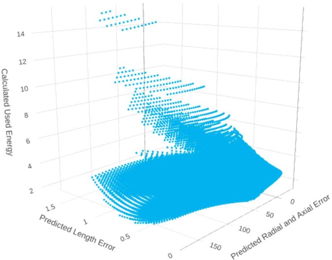

  

  Case Study 1: Predictions of metamodels iteration $k=1$. Note: Energy is calculated using Equation (21)

  The optimization method is implemented in Octave and ran in a PC (Intel i5-8250U, 1.6 GHz). Performing Step 1 and 2 of the optimization takes few seconds, so if we compared it with the time it will take to run thousands of simulations, metamodels are a very efficient way to represent simulation data for an optimization algorithm. Even for the best possible scenario of simulations taking only 30 minutes to compute, a similar global evaluation would need years of computational work to be done.

• 3. Find approximated Pareto Set and Front

  Now, the Pareto Front of the predicted solutions is found, it consist of 7257 solutions. Since the maximum number of simulations allowed per iteration $N_{\mathrm{sim}}^{\mathrm{max}} = 9$, 9 solutions were selected using a max-min distance criteria algorithm with 1000 iterations. This is, 1000 subsets of 9 points were randomly selected out of the 7257 points and the set for which the minimum distance between two points is the maximal was selected. The distances are calculated based on the input values (CPVs).

• 4. Evaluate selected predicted Pareto Solutions

  Table 3 shows the input and output values of the 9 new runs. Figures 10 and 11 show the input and output results as dark green circles.

  Figure 10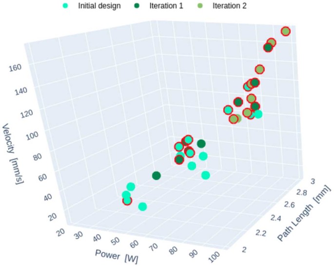

  

  Case Study 1: Values of controllable process variables for the initial experimental design (cyan), iteration $k=1$ (dark green) and iteration $k=2$ (olive green). The red circle around the dots mark the runs belonging to the final Pareto set

  Figure 11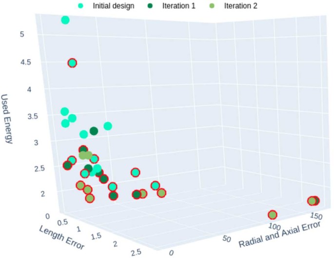

  

  Case Study 1: PMs values of initial experimental design (cyan), iteration $k=1$ (dark green) and iteration $k=2$ (olive green). The red circle around the dots mark the runs belonging to the final Pareto front

  Table 3 Case Study 1: Evaluation of selected predicted Pareto solutions and derived quantities, iterations $k=1$ (runs 16–24) and $k=2$ (runs 25–33)

• 5. Update Incumbent Pareto Front

  The incumbent Pareto Front is updated comparing the initial incumbent Pareto Front and the 9 additional runs. The new Pareto solutions are 1, 4, 7, 8, 12, 14, 15, 16, 18, 19, 21, 22, 23, and 24.

• 6. Evaluate Stopping Criteria

  Next, the stopping criteria are evaluated. The criteria used here are: (1) stop if the maximum number of simulations allowed was reached (no, $24 < 45$); (2) stop if $R^{2}$ of all models is larger than $1- \varepsilon=0.98$ (no, $R_{1}^{2} = 0.9673$ and $R_{2}^{2} = 0.9999$); (3) stop if no new Pareto solutions were found (no, new solutions were found). Since none of the stopping criteria were met, a new (main) iteration is needed.

On the second iteration, new metamodels were fitted using all available data (24 simulations). The $R^{2}$ of the new models are $R_{1}^{2}=0.9999$ and $R_{2}^{2}=0.9949$ respectively. Later, the models were used to predict a new Pareto front which had 2852 solutions, however only 9 were evaluated. The corresponding input and output values are shown on Table 3 (runs 25–33). Afterwards, the incumbent Pareto front was updated and the new Pareto solutions are 1, 4, 7, 8, 12, 14, 15, 16, 18, 19, 21, 22, 23, 24, 27–33. Then, the stopping criteria were evaluated and since the $R^{2}$ of both models are larger than 0.98 the method stopped and the final Pareto solutions are reported.

Report Final Incumbent Solutions

The final Pareto solutions are identified with an (^∗) next to the run number on Tables 2 and 3 and are marked with a red circle on Figs. 10 and 11.

This concludes the simulation-optimization procedure and delivers a set of solutions that represent the best compromises between all PMs. Now, practitioners can select the best one, depending on the current needs and the priorities they want to grant to each of the PMs.

4.3 Case study 2: optimization for shape and process efficiency

To further improve the laser-based material accumulation process, we now consider six objectives. Three PMs are related to shape quality and 3 more relevant to process efficiency. Objective 1 corresponds to minimize length error ($|\Delta l|$) [mm], objective 2 minimize radial error ($\Delta c_{xy}$) [μm], objective 3 minimize axial error ($\Delta c_{z}$) [μm], objective 4 minimize process time ($t_{\mathrm{ end}}$) [s], objective 5 minimize energy (E) [J] used and objective 6 minimize the laser usage time [ms]. Objectives 1, 2, 3 and 4 were measured as described in Sect. 1.2 and 2.4. Objectives 5 and 6 are calculated using equations (21) and (22) respectively.

$$ \text{laser usage}= \frac{s}{v} \times1000. $$

(22)

In this case study, the same CPVs of Case 1 were used. The range of the CPVs and fix variables was kept the same.

As in Case Study 1, the optimization was conducted following the flow chart in Fig. 7. The optimization parameters used here are: maximum number of simulations $N_{\mathrm{sim}}^{ \mathrm{total}} = 15 \times 6 = 90$; maximum number of simulations per iteration $N_{\mathrm{sim}}^{\mathrm{max}} = 3 \times 6 =18$; and the lower bound for $R^{2}$ was set again at 98% $(\varepsilon=0.02)$.

The initial design of experiments is the same as in Case Study 1. Table 4 shows the values of the CPVs and the corresponding PMs evaluations. The initial Pareto solutions are solutions 1–4, 6–8, 10–15.

Table 4 Case Study 2: Results of initial experimental design. A star in the first column indicates that it is a final Pareto solution

After the initial data is collected, a MLR model was fitted to estimate objectives 1 to 4 and objectives 5 and 6 were calculated using equations (21) and (22) respectively.

The $R^{2}$ of the four metamodels are 0.96729, 0.99866, 0.95088, and 0.99997, respectively. Then, the PM values of 157,781 solutions were estimated (see Case Study 1, main iteration, Step 2 as reference) and the predicted Pareto Front was identified. The predicted Pareto Front at iteration $k=1$ had 46,708 solutions, however only 18 were simulated. The selection was performed as in Case Study 1. Solutions 16 to 33 on Table 5 show the corresponding input and output values. The incumbent Pareto front is then updated and the new Pareto solutions are 1–4, 6–8, 10–16, 18–33. Since, none of the stopping criteria are met a new iteration began.

Table 5 Case Study 2: Evaluation of selected predicted Pareto solutions. Iterations are divided by horizontal lines. Iteration 1: solutions 16 to 33, Iteration 2: 33 to 51, Iteration 3: 52 to 69

A total of 3 iterations and 69 simulation runs were performed until the method stopped. Table 5 shows the results of the additional runs. Solutions 16 to 33 are for iteration 1, 34 to 51 for iteration 2, and 52 to 69 from iteration 3. The methods stopped because the $R^{2}$ of all metamodels was larger that the lower limit.

The final Pareto solutions correspond to simulation runs 1, 2, 4, 6–8, 11–15, 18–28, 30–33, 35–38, 40, 42, 44, 46–51, 53–62, 64, 65, 67–69 and are marked by an (^∗) next to the solution number on Tables 4 and 5.

The final Pareto Set is shown graphically on Figs. 12. It is denoted by the red circled solutions.

Figure 12

Case Study 2: Values of CPV for the initial experimental design (cyan), iteration $k=1$ (dark green), iteration $k=2$ (olive green), and iteration $k=3$ (yellow). The red circle around the dots mark the runs belonging to the final Pareto set

4.4 Comments on the optimization results

For Case Study 1 (Sect. 4.2), we have chosen two PMs for measuring the shape quality of the produced components and one more for the used energy needed on the process. It is important to mention that a process with correct molten length can be achieved by choosing an appropriate velocity v for a laser power P and path length s given within the CPVs feasible region. Further, a fast moving laser with high power usually leads to better energy efficiency, since the time for heat transport in distant regions and boundary fluxes is shorter.

Looking at Tables 2 and 3, runs 21, 28 and 31 give the minimal values of energy. These runs are special, since the applied energy per unit length $\frac{P}{v}< {0.58}$ $\frac{\text{J}}{\text{mm}}$ is too low in order to establish the formation of a larger molten volume. Instead, only the region around the laser’s impinging spot is melting and solidifying shortly afterwards. The opposite side of the wire is never molten in this case, resulting in nearly no deformation with respect to the wire’s initial geometry. Regarding the other two PMs, this is reflected by a non absolute value $\Delta l< {-2.37}$ mm and $\Delta c_{xyz}>{112.3}$ μm in which the latter is merely determined by the axial component.

A molten sphere is formed for $\frac{P}{v}>{0.66}$ $\frac {\text{J}}{\text{mm}}$ which is the case in all other runs. First we look at solutions with $l\leq s$ which correspond to runs 8, 12, 16, 22, 23, 29, 30 and 33. In these runs l is typically a bit smaller than s since solidification starts almost immediately after the laser is switched off. This prevents the melt from releasing it’s tilted shape as shown in Sect. 2.3 for Run 12.

With exception of Run 33, which is an extreme case with $l-s$ only being −0.046 mm, we have $\Delta c_{xyz}\in[28.42,81.51]$ for the shape error indicating now the strength of the final preform’s tilt. On the other hand we have the best energy efficiency in these runs with $\frac{l}{E}\geq {1.21}$ $\frac{\text{mm}}{\text{J}}$ (Run 33), which is worse for all other runs.

Further grouping regarding $\Delta c_{xyz}$ is difficult, since the discretization error for $\Delta c_{xyz}$ is typically ±10 μm for the underlying mesh but can go up to about 40 μm in worst cases as can be seen in Run 5. In general, the preform’s tilt and therefore $\Delta c_{xyz}$ decreases with increasing molten length over the laser path length $l-s$, which as a trade-off results in a worse $\frac{l}{E}$ ratio. The worst energy efficiency with $\frac{l}{E}\leq {1.0}$ $\frac{\text{J}}{\text{mm}}$ is achieved by Runs 1, 2, 5, 9, 11 and 13 for which we have $l-s>{0.44}$ mm and, due to numerical approximation errors, $\Delta c_{xyz}<{13.1}$ μm except for the aforementioned Run 5.

For Case 2 in Sect. 4.3, we considered the PMs of axial and radial errors separately (instead as the sum of them as in Case 1) and included two more PMs that are connected to the efficiency of the real process. In total, we have three geometrical PMs measuring the length, axial, and radial errors, complemented by efficiency PMs measuring the process time, used energy, and laser time.

It is remarkable how our optimization method succeeds in finding the Pareto front using metamodels reaching values of $R^{2}>0.98$ and avoiding the simulative effort for combinations of CPVs far away from the Pareto set.

The three dimensional visualizations in Fig. 13 show how for some points in the Pareto front, the values for a single PM might be very large. For example, the axial error shows some extremely large values, but these points are still part of the optimal solutions as they deliver values of almost zero length error and small values on the other four PMs.

Figure 13

Case Study 2: PMs values of initial experimental design (cyan), iteration $k=1$ (dark green), iteration $k=2$ (olive green), and iteration $k=3$ (yellow). The red circle around the dots mark the runs belonging to the final pareto front. Left: PMs 1, 2, and 3. Right: PMs 4, 5, and 6

Although it might be expected that the last three PMs are similar, the simulated cases have shown that the relations between their values are not easy to correlate. This might be confirmed observing the shape of the Pareto front regarding these three PMs in the left plot from Fig. 13, where no clear linear relation can be derived among the three PM values.

Analogous to Case 1, we have no formation of a molten sphere for $\frac{P}{v}<{0.65}$ $\frac{\text{J}}{\text{mm}}$ in runs 20, 31, 44, 47, 53, 56, 58, 64 and 69. This is reflected best by the axial error $\Delta c _{z}>{227.3}$ μm, for which in all other runs $\Delta c_{z}< {26.0}$ μm holds. Further, $l-s<0$ holds for runs 8, 12, 21, 23, 29, 38, 40, 42, 50, 51, 54, 55, 57, 59, 61, 62, 63, 65 and 68. Here we have again the best energy efficiency with $\frac{l}{E}\geq {1.22}$ $\frac{\text{mm}}{\text{J}}$ and $\Delta c_{xy}$ lies, except for runs 40, 42, 51 and 68, within $[30.6,101.2]$ indicating the preform’s tilt. Least energy efficiency with $\frac{l}{E}\leq {1.0}$ ${\frac {\text{J}}{\text{mm}}}$ is achieved by runs 1, 2, 5, 9, 11, 13, 17, 45, 49, 52 and 60 yielding $l-s>{0.62}$ mm and $\Delta c_{xy}<{21.1}$ μm with exception of Run 5.

4.5 Relation of metamodel output to experimental results

We want to relate our metamodel output to the experimental results mentioned already at the beginning of this section. $v_{\mathrm { opt}}$, given by (17), has been determined from several experiments in which $l\approx s$ holds. Hence, we should have $|\Delta l|\approx0$ for $s={3.0}$ mm. In the following, we will relate our results from Case study 2 close to $s={3.0}$ mm to $v_{\mathrm{ opt}}$ by considering Pareto solutions with $s\in[{2.8}~{\text{mm}}, {3.0}~{\text{mm}}]$ and metamodels for several PMs evaluated at $s={3.0}$ mm.

The simulation’s ability to reproduce experimental results is shown in the right plot of Fig. 14. As mentioned before, $|\Delta l|\approx0$ should be observed for all pairs $(P,v)$ of simulated Pareto solutions with s being close to 3.0 mm. For the simulated pairs $(P,v)$ with small values of $|\Delta l|$, in almost any case the velocity v is smaller than $v_{\mathrm{ opt}}$. This is on the one hand due to $s<{3.0}$ mm in most cases and on the other hand due to the systematic underestimation of l in the numerical approach. Overall, simulation results are in good agreement with experimental results.

Figure 14

Case Study 2. Left: Predicted Length error [mm] at $s=3.0$ mm using last metamodel (iteration $k=3$). Right: Length Error of Final Pareto Solutions with $s \geq2.8$ mm. In both cases, the length error is shown as indicated by the color bar and the solid line corresponds to $v_{\mathrm{ opt}}$

Further, the metamodel can be used to predict the value of PMs for CPV values that have not been simulated. Of course, the prediction quality depends on the distribution of CPVs during optimization. Exemplary, the left plot in Fig. 14 shows the metamodel prediction for different pairs $(P,v)$ with a fixed values of $s={3.0}$ mm. At this stage it is important to notice that the metamodels purely rely on the known values coming from simulated CPVs combinations. In this sense, they achieve very good fits in the areas where the objectives have dominant solutions, it is, close to the Pareto set. Nevertheless, the predicted values from the metamodels might show very large and even unrealistic values when evaluated at CPVs far away from the Pareto set.

In the left plot of Fig. 15 the radial error $|\Delta c_{xy}|$ is shown for the same Pareto solutions as before, which is generally increasing for decreasing energy per unit length $P/v$. The only exception for this is, if $P/v$ is too low to establish the formation of a molten sphere. In this case we have $|\Delta c_{xy}| \approx0$ but we have $|\Delta c_{z}|\gg0$ for the axial error as shown in the right plot of Fig. 15.

Figure 15

Case Study 2: Radial Error (left) and Axial Error (right) of Final Pareto Solutions with $s \geq2.8$ mm. The color of each dot indicates the radial and axial error, respectively. Solid line corresponds to $v_{\mathrm{opt}}$

Finally, we take a look at Process time, which is the only efficiency related PM we have that requires a metamodel. Figure 16 contains the predicted process time values using the metamodel and the values of the computed process time for the simulated points belonging to the Pareto set with $s > 2.8\text{ mm}$. It can be seen that Process time is highly correlated to the signed distance to the $v_{\mathrm{ opt}}$ line. The physical interpretation for this is, that overheating the melt above the melting temperature has the most significant impact on the overall process time since melting continues after laser switch-off and subsequent solidification is slower. Furthermore, a high laser power coupled with a corresponding high velocity generally results in a short duration of laser heating and hence a shorter Process time. However, the impact is less significant compared to the effect of overheating.

Figure 16

Case Study 2. Left: Predicted Process time [s] at $s=3.0$ mm using last metamodel (iteration $k=3$). Right: Process Time of Final Pareto Solutions with $s \geq= 2.8$ mm. In both cases, the process time is shown as indicated by the the color bars and the solid line corresponds to $v_{opt}$

5 Summary and conclusion

In this work we have dealt with the simulation based optimization for a material accumulation process. Starting with a general description of our simulation strategy based on physical models for the solid-liquid phase change and the corresponding changes in the geometrical shape of a three-dimensional domain, we presented the details of a new combination of numerical methods to conduct a FEM simulation solving for temperature, evolution of solid-liquid interphase, and also the moving boundaries of the time dependent 3d domain, that is capable to deal with various geometric and topological changes which may happen due to a large range of process parameters.

Further, the optimization method has been described, defining the precise steps to construct an efficient optimization procedure with results for multiple objectives by maintaining only a relatively small amount of FEM simulations. Our method is based on the use of a sequential surrogate modeling that makes use of few simulation results to emulate a general description of the mapping between CPVs and PMs.

We presented the results of applying our methodology to two case studies by considering first three and then six different PMs. The goal was to find the CPVs that optimize all of the defined PMs simultaneously. In general, the method was able to approximate a Pareto Front keeping only a modest number of computed FEM simulations, which is critical for the cases of interest where a single simulation or experimental run needs up to 10 hours to be computed.

Specially, for the second case study, we managed to solve a six dimensional variable space computing only 69 simulations. This might be considered from the perspective of the so called curse of dimensionality in which one might think that on a six-dimensional space approximated by only two points in each dimension, there is a total of $2^{6}=64$ points. But describing any function in a single dimension by using only two points leaves plenty of possibilities out of the analysis. Statistically speaking, analyzing a higher dimensional space requires a sampling of the searching space that grows exponentially with the dimension. However, we managed to construct a full search of the space by using only 69 evaluations.

In both case studies we finish the process with a fixed set of optimal soutions that might be used by the practitioners to select during the setup of a real process. In the future, we would like to consider how to account uncertainty on the Pareto front and use it as an additional factor on the decision making process.

Furthermore, we were able to connect the resulting values of our metamodels with already published experimental data where a linear relation of efficient combinations of laser power and velocity was found, cf. Figs. 14 and 15. This shows not only that the simulation offers a good fit with the experiments, but also that the metamodels can be used to describe the experimental values as well.

The optimization of industrial processes via physical models and numerical methods involves typically the solution of coupled systems of (nonlinear) equations. For our application, we have to cope with a coupled system of nonlinear PDEs in 3d, where the time dependent domain is part of the solution. For the optimization procedure, a rather wide range of process parameters has to be studied and the numerical method has to be robust in order to give reasonable results for all admissible sets of parameters. We presented a numerical method that is based on variational principles, especially for the free capillary surface of the liquid subdomain, and is able to derive performance measures for all admissible parameters. Nevertheless, time-dependent 3d simulations consume quite a lot of computing time. Here, the chosen optimization method based on meta-models is able to derive solutions for the multi-objective optimization problem with only very few actual simulations necessary. The framework presented in the previous chapters demonstrates that it is possible to optimize processes involving complex scenarios and corresponding numerical simulations while using only a reasonable amount of computing time. Additionally, the experiments show quite robust results of the optimization method, even with non-smooth data from numerical (discretized) simulations.

References

Bänsch E. Finite element discretization of the Navier–Stokes equations with a free capillary surface. Numer Math. 2001;88(2):203–35. https://doi.org/10.1007/PL00005443.
Bänsch E, Schmidt A. Free boundary problems in fluids and materials. In: Bonito A, Nochetto RH, editors. Geometric partial differential equations – part I. Handbook of numerical analysis. vol. 21. Elsevier; 2020. p. 555–619.
Barton RR. Simulation optimization using metamodels. In: Proc. winter simulation conference. 2009. p. 230–8. https://doi.org/10.1109/WSC.2009.5429328.
Binois M, Ginsbourger D, Roustant O. Quantifying uncertainty on Pareto fronts with Gaussian process conditional simulations. Eur J Oper Res. 2015;243(2):386–94. https://doi.org/10.1016/j.ejor.2014.07.032.
Brüning H. Prozesscharakteristiken des thermischen Stoffanhäufens in der Mikrofertigung. Ph.D. thesis. Universität Bremen; 2016. http://nbn-resolving.de/urn:nbn:de:gbv:46-00105713-11.
Brüning H, Jahn M, Vollertsen F, Schmidt A. Influence of laser beam absorption mechanism on eccentricity of preforms in laser rod end melting. In: Proc. 11th int. conf. on micro manufacturing, orange county. CA, USA. 2016. Paper #77.
Brüning H, Veenaas S, Vollertsen F. Determination of axial velocity of material accumulation in laser rod end melting process. In: Fang F, Brinksmeier E, Riemer O, editors. Proc. 4th int. conf. on nanomanufacturing (nanoMan 2014). 2014. p. 8–10.
Dong S, Chunsheng E, Fan B, Danai K, Kazmer DO. Process-driven input profiling for plastics processing. J Manuf Sci Eng. 2007;129(4):802–9.
Dziuk G. An algorithm for evolutionary surfaces. Numer Math. 1991;58:603–11.
Ehrgott M. Multicriteria optimization. Berlin: Springer; 2005. https://doi.org/10.1007/3-540-27659-9.
Elliott CM. On the finite element approximation of an elliptic variational inequality arising from an implicit time discretization of the Stefan problem. IMA J Numer Anal. 1981;1(1):115–25. https://doi.org/10.1093/imanum/1.1.115.
Hirt C, Nichols B. Volume of fluid (VOF) method for the dynamics of free boundaries. J Comput Phys. 1981;39:201–25.
Hoppe H. Progressive meshes. In: Proc. 23rd ann. conf. computer graphics and interactive techniques, SIGGRAPH’96. New York: ACM; 1996. p. 99–108. https://doi.org/10.1145/237170.237216.
Hung TC, Chan KY. Uncertainty quantifications of Pareto optima in multiobjective problems. J Intell Manuf. 2013;24(2):385–95. https://doi.org/10.1007/s10845-011-0602-9.
Jin R, Chen W, Sudjianto A. On sequential sampling for global metamodeling in engineering design. In: ASME 2002 International Design Engineering Technical Conferences and Computers and Information in Engineering Conference. American Society of Mechanical Engineers; 2002. p. 539–548.
Kok SW, Tapabrata R. A framework for design optimization using surrogates. Eng Optim. 2005;37(7):685–703. https://doi.org/10.1080/03052150500211911.
Li YF, Ng SH, Xie M, Goh TN. A systematic comparison of metamodeling techniques for simulation optimization in decision support systems. Appl Soft Comput. 2010;10(4):1257–73. https://doi.org/10.1016/j.asoc.2009.11.034.
Luttmann A. Modellierung und Simulation von Prozessen mit fest-flüssig Phasenübergang und freiem Kapillarrand. Ph.D. thesis. Universität Bremen; 2018. http://nbn-resolving.de/urn:nbn:de:gbv:46-00106445-14.
Montalvo-Urquizo J, Niebuhr C, Schmidt A, Villarreal-Marroquin M. Reducing deformation, stress and tool wear during milling processes using simulation-based multiobjective optimization. Int J Adv Manuf Technol. 2018;96:1859–73.
Sethian JA, Smereka P. Level set methods for fluid interfaces. Annu Rev Fluid Mech. 2003;35:341–72. https://doi.org/10.1146/annurev.fluid.35.101101.161105.
Si H. TetGen, a Delaunay-based quality tetrahedral mesh generator. ACM Trans Math Softw. 2015;41(2):11:1–11:36. https://doi.org/10.1145/2629697.
Sussman M, Smereka P, Osher S. A level set approach for computing solutions to incompressible two-phase flow. J Comput Phys. 1994;114(1):146–59.
Villarreal-Marroquin MG, Cabrera-Rios M, Castro JM. A multicriteria simulation optimization method for injection molding. J Polym Eng. 2011;31(5):397–407.
Villarreal-Marroquin MG, Po-Hsu C, Mulyana R, Santner TJ, Dean AM, Castro JM. Multiobjective optimization of injection molding using a calibrated predictor based on physical and simulated data. Polym Eng Sci. 2016;57(3):248–57.
Villarreal-Marroquin MG, Svenson JD, Sun F, Santner TJ, Dean AM, Castro JM. A comparison of two metamodel-based methodologies for multiple criteria simulation optimization using an injection molding case study. J Polym Eng. 2013;33(3):193–209.
Vollertsen F. Categories of size effects. Prod Eng Res Dev. 2008;2(4):377–83. https://doi.org/10.1007/s11740-008-0127-z.
Wang GG, Shan S. Review of metamodeling techniques in support of engineering design optimization. J Mech Des. 2007;129(4):370–80.
Welch SWJ, Wilson J. A volume of fluid based method for fluid flows with phase change. J Comput Phys. 2000;160(2):662–82. https://doi.org/10.1006/jcph.2000.6481.
Zhou H. Computer modeling for injection molding: simulation, optimization, and control. New York: Wiley; 2012.
Acknowledgements
We thank the Bremer Institut für angewandte Strahltechnik for cooperation and the unknown referees for valuable remarks and suggestions.
Availability of data and materials
Not applicable.
Funding
The authors gratefully acknowledge the financial support by the DFG (German Research Foundation) for the subproject A3 within the Collaborative Research Center SFB 747 “Mikrokaltumformen—Prozesse, Charakterisierung, Optimierung”.
Author information
Authors and Affiliations
Contributions
FEM was developed in Bremen and Erlangen by EB, AL, and AS, simulations were performed in Bremen by AL and AS, the optimization method was conducted in Monterrey by JMU and MGVM. All authors contributed to the discussion of results and the manuscript text. All authors read and approved the final manuscript.
Corresponding author
Ethics declarations
Competing interests
The authors declare that they have no competing interests.
Additional information
Publisher’s Note
Springer Nature remains neutral with regard to jurisdictional claims in published maps and institutional affiliations.
Rights and permissions
Open Access This article is licensed under a Creative Commons Attribution 4.0 International License, which permits use, sharing, adaptation, distribution and reproduction in any medium or format, as long as you give appropriate credit to the original author(s) and the source, provide a link to the Creative Commons licence, and indicate if changes were made. The images or other third party material in this article are included in the article’s Creative Commons licence, unless indicated otherwise in a credit line to the material. If material is not included in the article’s Creative Commons licence and your intended use is not permitted by statutory regulation or exceeds the permitted use, you will need to obtain permission directly from the copyright holder. To view a copy of this licence, visit http://creativecommons.org/licenses/by/4.0/.
About this article
Cite this article
Bänsch, E., Luttmann, A., Montalvo-Urquizo, J. et al. Simulation and multi-objective optimization to improve the final shape and process efficiency of a laser-based material accumulation process. J.Math.Industry 10, 2 (2020). https://doi.org/10.1186/s13362-020-0070-y
Received:
Accepted:
Published:
DOI: https://doi.org/10.1186/s13362-020-0070-y